如何扩展你的模型(5):如何并行训练一个 Transformer
中英对照第 5 篇:FSDP / ZeRO、Megatron 张量并行、流水线并行、专家并行——给定芯片数和 batch size,怎样组合这些技术把训练效率做到最高。左栏原文,右栏译文。
本篇属于系列 如何扩展你的模型(How To Scale Your Model) · 第 5 篇
原文:How To Scale Your Model(Google DeepMind,作者 Jacob Austin、Sholto Douglas、Roy Frostig、Anselm Levskaya、Charlie Chen、Sharad Vikram、Federico Lebron、Peter Choy、Vinay Ramasesh、Albert Webson、Reiner Pope)。
本站是中英对照排版:左栏是英文原文,右栏是对应的中文译文。不好直译的术语(roofline、strong scaling、ICI、MXU、KV cache、FSDP、TP 等)保留英文写法;原文配图全部保留。
本文是系列《如何扩展你的模型(How To Scale Your Model)》的第 5 篇,共 13 篇。系列目录。
原文以 MIT 许可证发布,版权归 Google LLC;本译文仅作学习交流之用,如有错漏以原文为准。
What Do We Mean By Scaling?
「扩展」到底指什么?
The goal of “model scaling” is to be able to increase the number of chips used for training or inference while achieving a proportional, linear increase in throughput (we call this strong scaling). While performance on a single chip depends on the trade-off between memory bandwidth and FLOPs, performance at the cluster level depends on hiding inter-chip communication by overlapping it with useful FLOPs. This is non-trivial, because increasing the number of chips increases the communication load while reducing the amount of per-device computation we can use to hide it. As we saw in Section 3, sharded matrix multiplications often require expensive AllGathers or ReduceScatters that can block the TPUs from doing useful work. The goal of this section is to find out when these become too expensive.
「模型扩展」(model scaling)的目标,是在增加用于训练或推理的芯片数量的同时,让吞吐量也成比例地线性增长(我们称之为 strong scaling,强扩展)。单芯片上的性能取决于显存带宽与 FLOPs 之间的取舍;而集群层面的性能,则取决于能否用有用的 FLOPs 把芯片间通信掩盖(overlap)掉。这件事并不容易:芯片越多,通信负载越大,而能用来掩盖通信的每设备计算量反而越少。正如第 3 节所见,分片矩阵乘法往往需要昂贵的 AllGather 或 ReduceScatter,它们会挡住 TPU 去做有用的工作。本节的目标就是搞清楚:这些通信什么时候会变得过于昂贵。
In this section, we’ll discuss four common parallelism schemes: (pure) data parallelism, fully-sharded data parallelism (FSDP / ZeRO sharding), tensor parallelism (also known as model parallelism), and (briefly) pipeline parallelism. For each, we’ll show what communication cost we incur and at what point that cost starts to bottleneck our compute cost. (We’ll focus on communication bounds — since while memory capacity constraints are important, they typically do not bound us when using rematerialization (activation checkpointing) and a very large number of chips during pre-training. We also do not discuss expert parallelism here for MoEs — which expands the design space substantially, only the base case of a dense Transformer.) For this section, you can focus solely on inter-chip communication costs, since as long as we have a large enough single-chip batch size, the transfer of data from HBM to MXU is already overlapped with computation.
本节我们会讨论四种常见的并行方案:(纯)数据并行、完全分片数据并行(FSDP / ZeRO 分片)、张量并行(也叫模型并行),以及(简要提及)流水线并行。对每一种,我们都会说明它带来多少通信开销,以及这个开销从什么时候开始成为计算开销的瓶颈。(我们重点关注通信瓶颈——因为虽然显存容量约束也很重要,但在预训练中只要用上重算 / rematerialization(激活检查点)和足够多的芯片,容量通常不会成为瓶颈。这里也不讨论 MoE 的专家并行——它会显著扩大设计空间,我们只考虑稠密 Transformer 的基础情形。)在本节里,你可以只关注芯片间通信开销:只要单芯片上的 batch size 足够大,HBM 到 MXU 的数据搬运本身已经被计算掩盖了。
We’ll use the following notation to simplify calculations throughout this section.
为简化本节的计算,我们使用如下记号。
| Notation | Meaning (model parameters) |
|---|---|
| D | dmodel (the hidden dimension/residual stream dim) |
| F | dff (the feed-forward dimension) |
| B | Batch dimension (number of tokens in the batch; total, not per-device) |
| T | Sequence length |
| L | Number of layers in the model |
| 记号 | 含义(模型参数) |
|---|---|
| D | dmodel(隐藏维度 / 残差流维度) |
| F | dff(前馈维度) |
| B | Batch 维度(batch 中的 token 数;是总数,不是每设备的数量) |
| T | 序列长度 |
| L | 模型层数 |
| Notation | Meaning (hardware characteristic) |
|---|---|
| C | FLOPS/s per chip |
| W | Network bandwidth (bidirectional, often subscripted as e.g. $W_{\text{ici}}$ or $W_{\text{dcn}}$) |
| X | Number of chips along mesh axis X |
| Y | Number of chips along an alternate mesh axis, labeled Y |
| Z | Number of chips along a third mesh axis, labeled Z |
| 记号 | 含义(硬件特性) |
|---|---|
| C | 每芯片 FLOPS/s |
| W | 网络带宽(双向,常带下标,例如 $W_{\text{ici}}$ 或 $W_{\text{dcn}}$) |
| X | 沿 mesh 轴 X 的芯片数 |
| Y | 沿另一条 mesh 轴(记为 Y)的芯片数 |
| Z | 沿第三条 mesh 轴(记为 Z)的芯片数 |
For simplicity’s sake, we’ll approximate a Transformer as a stack of MLP blocks — attention is a comparatively small fraction of the FLOPs for larger models as we saw in Section 4. We will also ignore the gating matmul, leaving us with the following simple structure for each layer:
为简单起见,我们把 Transformer 近似成一摞 MLP 块——如第 4 节所示,对较大的模型来说,注意力只占 FLOPs 中相对很小的一部分。我们还会忽略 gating matmul,于是每一层就简化成下面这个结构:
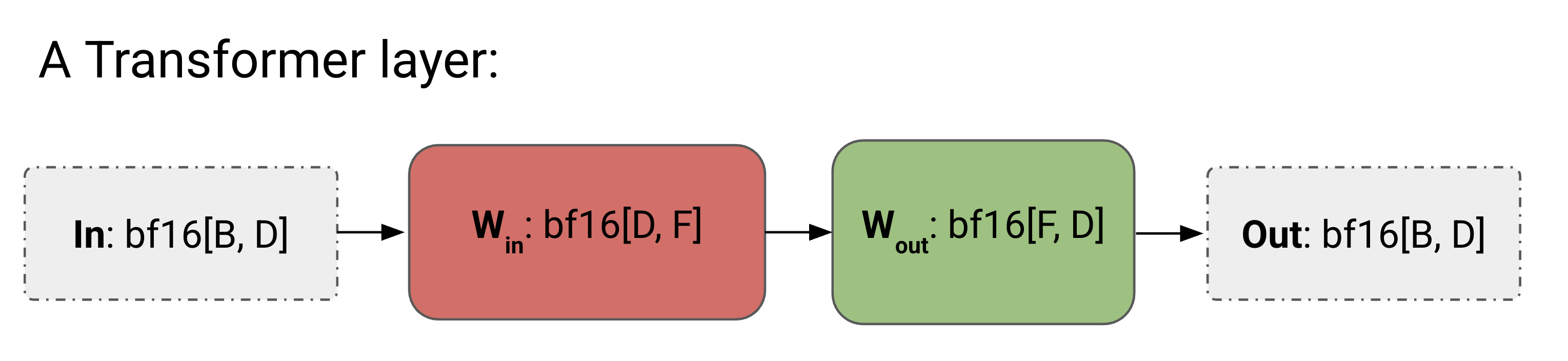
bf16[D, F] (up-projection) and Wout: bf16[F, D] (down-projection) with an input In: bf16[B, D].Here's the full algorithm for our little Transformer with no parallelism.
下面是我们这个没有任何并行的小 Transformer 的完整算法。
Forward pass: need to compute Loss[B]
前向传播: 需要计算 Loss[B]
- Tmp[B, F] = In[B, D] *D Win[D, F]
- Out[B, D] = Tmp[B, F] *F Wout[F, D]
- Loss[B] = …
Backward pass: need to compute dWout[F, D], dWin[D, F]
反向传播: 需要计算 dWout[F, D]、dWin[D, F]
- dOut[B, D] = …
- dWout[F, D] = Tmp[B, F] *B dOut[B, D]
- dTmp[B, F] = dOut[B, D] *D Wout[F, D]
- dWin[D, F] = In[B, D] *B dTmp[B, F]
- dIn[B, D] = dTmp[B, F] *F Win[D, F] (needed for previous layers)
- dOut[B, D] = …
- dWout[F, D] = Tmp[B, F] *B dOut[B, D]
- dTmp[B, F] = dOut[B, D] *D Wout[F, D]
- dWin[D, F] = In[B, D] *B dTmp[B, F]
- dIn[B, D] = dTmp[B, F] *F Win[D, F](前面几层需要用到)
We provide this for comparison to the algorithms with communication added.
我们给出它,是为了和后面加入通信的算法做对比。
Here are the 4 parallelism schemes we will discuss. Each scheme can be thought of as uniquely defined by a sharding for In, Win, Wout, and Out in the above diagram.
下面是我们将要讨论的 4 种并行方案。每一种都可以看作是在上图里对 In、Win、Wout 和 Out 采用了一种独特的分片方式。
1. Data parallelism: activations sharded along batch, parameters and optimizer state are replicated on each device. Communication only occurs during the backwards pass.
1. 数据并行: 激活沿 batch 分片,参数和优化器状态在每台设备上复制一份。通信只发生在反向传播期间。
$$\text{In}[B_X, D] \cdot_D W_\text{in}[D, F] \cdot_F W_\text{out}[F, D] \rightarrow \text{Out}[B_X, D]$$
2. Fully-sharded data parallelism (FSDP or ZeRO-3): activations sharded along batch (like pure data parallelism), parameters sharded along same mesh axis and AllGathered just-in-time before use in forward pass. Optimizer state also sharded along batch. Reduces duplicated memory.
2. 完全分片数据并行(FSDP 或 ZeRO-3): 激活沿 batch 分片(和纯数据并行一样),参数沿同一条 mesh 轴分片,并在前向传播用到之前即时 AllGather。优化器状态也沿 batch 分片。减少了重复的显存占用。
$$\text{In}[B_X, D] \cdot_D W_\text{in}[D_X, F] \cdot_F W_\text{out}[F, D_X] \rightarrow \text{Out}[B_X, D]$$
3. Tensor parallelism (also called Megatron sharding or model parallelism): activations sharded along D ($d_\text{model}$), parameters sharded along F ($d_{ff}$). AllGather and ReduceScatter activations before and after each block. Compatible with FSDP.
3. 张量并行(也叫 Megatron 分片或模型并行): 激活沿 D($d_\text{model}$)分片,参数沿 F($d_{ff}$)分片。在每个块的前后对激活做 AllGather 和 ReduceScatter。可与 FSDP 组合。
$$\text{In}[B, D_Y] \cdot_D W_\text{in}[D, F_Y] \cdot_F W_\text{out}[F_Y, D] \rightarrow \text{Out}[B, D_Y]$$
4. Pipeline parallelism: weights sharded along the layer dimension, activations microbatched and rolled along the layer dimension. Communication between pipeline stages is minimal (just moving activations over a single hop). To abuse notation:
4. 流水线并行: 权重沿层的维度分片,激活被切成微批(microbatch)并沿层维度滚动传递。流水线各阶段之间的通信极少(只是把激活沿单跳搬运一下)。为了偷懒,滥用一下记号:
$$\text{In}[L_Z, B, D][i] \cdot_D W_\text{in}[L_Z, D, F][i] \cdot_F W_\text{out}[L_Z, F, D][i] \rightarrow \text{Out}[L_Z, B, D][i]$$
Data Parallelism
数据并行
Syntax: $$\text{In}[B_X, D] \cdot_D W_\text{in}[D, F] \cdot_F W_\text{out}[F, D] \rightarrow \text{Out}[B_X, D]$$
写法: $$\text{In}[B_X, D] \cdot_D W_\text{in}[D, F] \cdot_F W_\text{out}[F, D] \rightarrow \text{Out}[B_X, D]$$
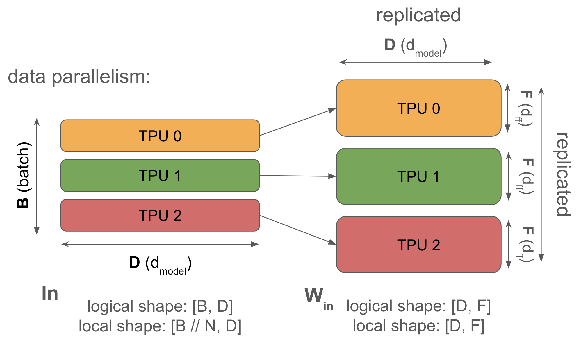
When your model fits on a single chip with even a tiny batch size (>240 tokens, so as to be compute-bound), you should always use simple data parallelism. Pure data parallelism splits our activations across any number of TPUs so long as the number of TPUs is smaller than our batch size. The forward pass involves no communication, but at the end of every step, each TPU performs an AllReduce on its local gradients to synchronize them before updating the parameters.
只要你的模型能装进单颗芯片,哪怕 batch size 很小(>240 个 token,以便保持计算受限),你都应该优先用简单的数据并行。 纯数据并行把激活切分到任意多颗 TPU 上,只要 TPU 数量小于 batch size 即可。前向传播不涉及任何通信,但在每一步结束时,每颗 TPU 会对自己本地的梯度做一次 AllReduce,在更新参数前把它们同步起来。
Here's the full algorithm for the forward and backwards pass. We abuse notation to write dL/dOut as dOut, purely for compactness.
下面是前向和反向传播的完整算法。为了简洁,我们滥用记号,把 dL/dOut 写成 dOut。
Pure Data Parallelism Algorithm:
纯数据并行算法:
Forward pass: need to compute Loss[BX]
前向传播: 需要计算 Loss[BX]
- Tmp[BX, F] = In[BX, D] *D Win[D, F]
- Out[BX, D] = Tmp[BX, F] *F Wout[F, D]
- Loss[BX] = …
Backward pass: need to compute dWout[F, D], dWin[D, F]
反向传播: 需要计算 dWout[F, D]、dWin[D, F]
- dOut[BX, D] = …
- dWout[F, D] {UX} = Tmp[BX, F] *B dOut[BX, D]
- dWout[F, D] = AllReduce(dWout[F, D] {UX}) (not on critical path, can be done async)
- dTmp[BX, F] = dOut[BX, D] *D Wout[F, D]
- dWin[D, F] {UX} = In[BX, D] *B dTmp[BX, F]
- dWin[D, F] = AllReduce(dWin[D, F] {UX}) (not on critical path, can be done async)
- dIn[BX, D] = dTmp[BX, F] *F Win[D, F] (needed for previous layers)
- dOut[BX, D] = …
- dWout[F, D] {UX} = Tmp[BX, F] *B dOut[BX, D]
- dWout[F, D] = AllReduce(dWout[F, D] {UX})(不在关键路径上,可以异步做)
- dTmp[BX, F] = dOut[BX, D] *D Wout[F, D]
- dWin[D, F] {UX} = In[BX, D] *B dTmp[BX, F]
- dWin[D, F] = AllReduce(dWin[D, F] {UX})(不在关键路径上,可以异步做)
- dIn[BX, D] = dTmp[BX, F] *F Win[D, F](前面几层需要用到)
We ignore the details of the loss function and abbreviate $\text{Tmp} = W_\text{in} \cdot \text{In}$. Note that, although our final loss is the average AllReduce(Loss[BX]), we only need to compute the AllReduce on the backward pass when averaging weight gradients.
我们忽略损失函数的具体细节,并把 $\text{Tmp} = W_\text{in} \cdot \text{In}$ 记作 Tmp。注意,虽然最终的 loss 是 AllReduce(Loss[BX]) 的平均,但在反向传播里我们只在平均权重梯度时才需要做 AllReduce。
Note that the forward pass has no communication — it’s all in the backward pass! The backward pass also has the great property that the AllReduces aren’t in the “critical path”, meaning that each AllReduce can be performed whenever it’s convenient and doesn’t block you from performing subsequent operations. The overall communication cost can still bottleneck us if it exceeds our total compute cost, but it is much more forgiving from an implementation standpoint. We’ll see that model/tensor parallelism doesn’t have this property.
注意前向传播没有任何通信——通信全都在反向传播里!反向传播还有一个很棒的性质:这些 AllReduce 不在「关键路径」上,也就是说每次 AllReduce 可以在任意方便的时候做,不会挡住后续操作。如果总通信开销超过总计算开销,它仍然可能成为瓶颈,但从实现角度看它要宽容得多。后面我们会看到,模型 / 张量并行没有这个性质。
Why do this? Pure data parallelism reduces activation memory pressure by splitting our activations over the batch dimension, allowing us to almost arbitrarily increase batch size as long as we have more chips to split the batch dimension over. Especially during training when our activations often dominate our memory usage, this is very helpful.
为什么这么做? 纯数据并行把激活按 batch 维度切开,从而缓解激活带来的显存压力,也让我们只要有多余芯片去切分 batch 维度,就能近乎任意地增大 batch size。尤其在训练中,激活往往占据显存的大头,这一招非常有用。
Why not do this? Pure data parallelism does nothing to reduce memory pressure from model parameters or optimizer states, which means pure data parallelism is rarely useful for interesting models at scale where our parameters + optimizer state don’t fit in a single TPU. To give a sense of scale, if we train with parameters in bf16 and optimizer state in fp32 with Adam (Adam stores parameters, first order and second order accumulators. Since the params are in bfloat16 and optimizer state is in float32, this gives us 2 + 8 = 10 bytes per parameters.), the largest model we can fit has $$\text{TPU memory} / 10$$ parameters, so e.g. on a TPUv5p chip with 96GB of HBM and pure data parallelism this is about 9B parameters.
为什么不这么做? 纯数据并行完全不能缓解模型参数或优化器状态带来的显存压力,所以在参数量 + 优化器状态装不进单颗 TPU 的大规模场景下,纯数据并行几乎没用。给一个量级感:如果我们用 bf16 存参数、用 fp32 存 Adam 优化器状态(Adam 会保存参数、一阶和二阶累加器;参数是 bfloat16、优化器状态是 float32,于是每个参数占 2 + 8 = 10 字节),能装下的最大模型就是 $$\text{TPU memory} / 10$$ 个参数——比如在 HBM 为 96GB 的 TPUv5p 芯片上做纯数据并行,大约是 9B 参数。
Takeaway: the largest model we can train with Adam and pure data parallelism has $$\text{num\_params} = \text{HBM per device} / 10$$. For TPU v5p this is roughly 9B parameters. (Note that this doesn’t include gradient checkpoints, so this wouldn’t actually be useful. This is an absolute lower bound with a batch of 1 token.)
结论: 用 Adam 加纯数据并行能训练的最大模型有 $$\text{num\_params} = \text{HBM per device} / 10$$ 个参数。对 TPU v5p 来说大约是 9B 参数。(注意这还没算梯度检查点,所以实际上并不可用;这只是 batch 为 1 个 token 时的绝对下界。)
To make this useful for real models during training, we’ll need to at least partly shard the model parameters or optimizer.
要让它在真实模型的训练中真正有用,我们至少得把模型参数或优化器状态部分分片。
When do we become bottlenecked by communication? As we can see above, we have two AllReduces per layer, each of size $$2DF$$ (for bf16 weights). When does data parallelism make us communication bound?
我们什么时候会被通信卡住? 如上面所见,每一层有两次 AllReduce,每次的大小都是 $$2DF$$(对 bf16 权重而言)。数据并行在什么时候会让我们变成通信受限?
As in the table above, let $C$ = per-chip FLOPs, $W_{\text{ici}}$ = bidirectional network bandwidth, and $X$ = number of shards across which the batch is partitioned (We assume this partitioning is done over an ICI mesh, so the relevant network bandwidth is $W_\text{ici}$). Let’s calculate the time required to perform the relevant matmuls, $$T_\text{math}$$, and the required communication time $$T_\text{comms}$$. Since this parallelism scheme requires no communication in the forward pass, we only need to calculate these quantities for the backwards pass.
沿用上表的记号,设 $C$ = 每芯片 FLOPs,$W_{\text{ici}}$ = 双向网络带宽,$X$ = batch 被切分到的分片数(我们假设切分是在 ICI mesh 上做的,所以相关带宽是 $W_\text{ici}$)。我们来计算相关矩阵乘法所需的时间 $$T_\text{math}$$,以及通信所需的时间 $$T_\text{comms}$$。由于这种并行方案在前向传播中不需要通信,我们只需针对反向传播计算这两个量。
Communication time: From a previous section we know that the time required to perform an AllReduce in a 1D mesh depends only on the total bytes of the array being AllReduced and the ICI bandwidth $W_\text{ici}$; specifically the AllReduce time is $2 \cdot \text{total bytes} / W_\text{ici}$. Since we need to AllReduce for both $W_\text{in}$ and $W_\text{out}$, we have 2 AllReduces per layer. Each AllReduce is for a weight matrix, i.e. an array of $DF$ parameters, or $2DF$ bytes. Putting this all together, the total time for the AllReduce in a single layer is
通信时间: 从前面的章节我们知道,在 1D mesh 上做一次 AllReduce 所需的时间只取决于被 AllReduce 的数组总字节数和 ICI 带宽 $W_\text{ici}$;具体来说,AllReduce 时间是 $2 \cdot \text{总字节数} / W_\text{ici}$。由于 $W_\text{in}$ 和 $W_\text{out}$ 都需要 AllReduce,每一层共有 2 次 AllReduce。每次 AllReduce 针对一个权重矩阵,即 $DF$ 个参数、也就是 $2DF$ 字节的数组。把这些合起来,单层 AllReduce 的总时间是
$$\begin{align} T_\text{comms} &= \frac{2 \cdot 2 \cdot 2 \cdot D \cdot F}{W_\text{ici}}. \\ \end{align}$$
Matmul time: Each layer comprises two matmuls in the forward pass, or four matmuls in the backwards pass, each of which requires $2(B/X)DF$ FLOPs. Thus, for a single layer in the backward pass, we have
矩阵乘法时间: 每一层在前向传播中有两次矩阵乘法,反向传播中有四次,每次都需要 $2(B/X)DF$ 次 FLOPs。于是对反向传播中的单层,我们有
$$\begin{align} T_\text{math} &= \frac{2 \cdot 2 \cdot 2 \cdot B \cdot D \cdot F}{X \cdot C} \\ \end{align}$$
Since we overlap, the total time per layer is the max of these two quantities:
由于二者可以重叠,每层的总时间取这两个量的最大值:
$$\begin{aligned} T &\approx \max(\frac{8 \cdot B \cdot D \cdot F}{X \cdot C}, \frac{8 \cdot D \cdot F}{W_\text{ici}}) \\ T &\approx 8 \cdot D \cdot F \cdot \max(\frac{B}{X \cdot C}, \frac{1}{W_\text{ici}}) \end{aligned}$$
We become compute-bound when $$T_\text{math}/T_\text{comms} > 1$$, or when
当 $$T_\text{math}/T_\text{comms} > 1$$ 时,我们就变成计算受限,也就是当
$$\begin{align} \frac{B}{X} > \frac{C}{W_\text{ici}}. \end{align}$$
The upshot is that, to remain compute-bound with data parallelism, we need the per-device batch size $$B / X$$ to exceed the ICI operational intensity, $C / W_\text{ici}$. This is ultimately a consequence of the fact that the computation time scales with the per-device batch size, while the communication time is independent of this quantity (since we are transferring model weights). Note the resemblance of the $B/X > C/W_\text{ici}$ condition to the single-device compute-bound rule $B > 240$; in that case as well, the rule came from the fact that computation time scaled with batch size while data-transfer size was (in the $B \ll F, D$ regime) independent of batch size.
结论是:要想在数据并行下保持计算受限,每设备 batch size $$B / X$$ 必须超过 ICI 的算术强度 $C / W_\text{ici}$。归根结底,这是因为计算时间随每设备 batch size 增长,而通信时间与之无关(因为我们搬运的是模型权重)。注意 $B/X > C/W_\text{ici}$ 这个条件与单设备计算受限规则 $B > 240$ 很像;那里的规则同样源于「计算时间随 batch size 增长,而(在 $B \ll F, D$ 区间)数据传输量与 batch size 无关」。
Let’s put in some real numbers to get a sense of scale. For TPUv5p, C=4.6e14 and W=2 * 9e10 for 1D data parallelism over ICI, so our batch size per chip must be at least 2,550 to avoid being communication-bound. Since we can do data parallelism over multiple axes, if we dedicate all three axes of a TPUv5p pod to pure data parallelism, we 3x our bandwidth $W_\text{ici}$ and can scale down to only BS=850 per TPU or 7.6M tokens per batch per pod (of 8960 chips)! This tells us that it’s fairly hard to become bottlenecked by pure data parallelism!
代入一些真实数字来找找量级感。对 TPUv5p,在 ICI 上做 1D 数据并行时 C=4.6e14、W=2 * 9e10,所以每芯片的 batch size 至少要有 2,550,才能避免通信受限。由于我们可以沿多条轴做数据并行,如果把 TPUv5p pod 的三条轴全都用于纯数据并行,$W_\text{ici}$ 就变成三倍,可以低到每颗 TPU 只需 BS=850,即每个 pod(8960 颗芯片)每批 7.6M 个 token!这说明纯数据并行其实很难成为瓶颈!
Note [context parallelism]: Throughout this section, $B$ always refers to the total batch size in tokens. Clearly, however, our batch is made up of many different sequences, so how does this work? As far as the MLP is concerned, tokens are tokens! It doesn’t matter if they belong to the same sequence or two different sequences. So we are more or less free to do data parallelism over both the batch and sequence dimension: we call this context parallelism or sequence parallelism, but you can think of it as simply being another kind of data parallelism. Attention is trickier than the MLP since we do some cross-sequence computation, but this can be handled by gathering KVs or Qs during attention and carefully overlapping FLOPs and comms (typically using something called “ring attention”). Throughout this section, we will just ignore our sequence dimension entirely and assume some amount of batch or sequence parallelism.
注 [context parallelism(上下文并行)]: 本节中 $B$ 始终指以 token 计的总 batch size。但显然我们的 batch 由许多不同的序列组成,这要怎么处理?对 MLP 而言,token 就是 token!它属于同一条还是两条不同的序列都无所谓。所以我们差不多可以自由地同时沿 batch 和序列维度做数据并行:这被称为 context parallelism 或 sequence parallelism,但你可以把它简单理解成另一种数据并行。注意力比 MLP 更麻烦,因为其中有一些跨序列的计算,但这可以通过在注意力过程中收集 KV 或 Q,并小心地让 FLOPs 与通信重叠来处理(通常用的是所谓的「ring attention」)。本节中我们干脆完全忽略序列维度,假定已经做了某种 batch 或序列并行。
Note on multiple mesh axes: We should quickly note how multiple axes affects the available bandwidth. When we use multiple mesh axes for a given parallelism strategy, we get more bandwidth.
关于多条 mesh 轴的注记: 我们应该顺带说明多条轴如何影响可用带宽。当一种并行策略跨越多条 mesh 轴时,我们能获得更多带宽。
- Definition: $M_X$ ($M_Y$, $M_Z$, etc.) is the number of hardware mesh axes that a given parallelism strategy spans.
- Effect (bandwidth-bound): Using $M$ axes provides ($\approx M$ times) aggregate link bandwidth, so collective time scales $\propto 1/M_X$.
- 定义: $M_X$($M_Y$、$M_Z$ 等)是某种并行策略跨越的硬件 mesh 轴数。
- 效果(带宽受限时): 使用 $M$ 条轴会提供(约 $M$ 倍的)聚合链路带宽,于是集合通信时间按 $\propto 1/M_X$ 缩放。
Fully-Sharded Data Parallelism (FSDP)
完全分片数据并行(FSDP)
Syntax: $$\text{In}[B_X, D] \cdot_D W_\text{in}[D_X, F] \cdot_F W_\text{out}[F, D_X] \rightarrow \text{Out}[B_X, D]$$
写法: $$\text{In}[B_X, D] \cdot_D W_\text{in}[D_X, F] \cdot_F W_\text{out}[F, D_X] \rightarrow \text{Out}[B_X, D]$$
Fully-sharded data parallelism (often called FSDP or ZeRO-sharding[zero]) splits the model optimizer states and weights across the data parallel shards and efficiently gathers and scatters them as needed. Compared to pure data parallelism, FSDP drastically reduces per-device memory usage and saves on backward pass FLOPs, with very minimal overhead.
完全分片数据并行(常被称为 FSDP 或 ZeRO 分片[zero])把模型的优化器状态和权重切分到各个数据并行分片上,并按需高效地 gather / scatter。与纯数据并行相比,FSDP 大幅降低每设备显存占用,还节省反向传播的 FLOPs,而额外开销极小。
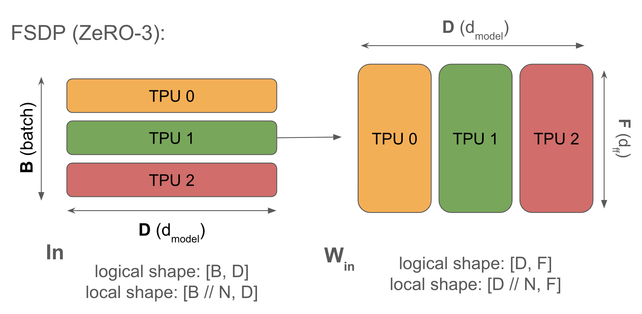
You’ll remember (from Section 3) that an AllReduce can be decomposed into an AllGather and a ReduceScatter. This means that, instead of doing the full gradient AllReduce for standard data parallelism, we can shard the weights and optimizer states across chips, AllGather them at each layer during the forward pass and ReduceScatter across the weights during the backward pass at no extra cost.
你应当记得(在第 3 节里),一次 AllReduce 可以分解成一次 AllGather 加一次 ReduceScatter。这意味着,标准数据并行里那次完整的梯度 AllReduce 可以换成:把权重和优化器状态分片到各芯片上,在前向传播中逐层 AllGather 权重,在反向传播中按权重 ReduceScatter——而总代价不变。
Here's the full algorithm for FSDP.
下面是 FSDP 的完整算法。
Fully-Sharded Data Parallelism (FSDP):
完全分片数据并行(FSDP):
Forward pass: need to compute Loss[BX]
前向传播: 需要计算 Loss[BX]
- Win[D, F] = AllGather(Win[DX, F]) (not on critical path, can do it during previous layer)
- Tmp[BX, F] = In[BX, D] *D Win[D, F] (can throw away Win[D, F] now)
- Wout[F, D] = AllGather(Wout[F, DX]) (not on critical path, can do it during previous layer)
- Out[BX, D] = Tmp[BX, F] *F Wout[F, D]
- Loss[BX] = …
- Win[D, F] = AllGather(Win[DX, F])(不在关键路径上,可以在上一层执行时顺手做)
- Tmp[BX, F] = In[BX, D] *D Win[D, F](现在可以把 Win[D, F] 丢掉)
- Wout[F, D] = AllGather(Wout[F, DX])(不在关键路径上,可以在上一层执行时顺手做)
- Out[BX, D] = Tmp[BX, F] *F Wout[F, D]
- Loss[BX] = …
Backward pass: need to compute dWout[F, DX], dWin[DX, F]
反向传播: 需要计算 dWout[F, DX]、dWin[DX, F]
- dOut[BX, D] = …
- dWout[F, D] {UX} = Tmp[BX, F] *B dOut[BX, D]
- dWout[F, DX] = ReduceScatter(dWout[F, D] {UX}) (not on critical path, can be done async)
- Wout[F, D] = AllGather(Wout[F, DX]) (can be done ahead of time)
- dTmp[BX, F] = dOut[BX, D] *D Wout[F, D] (can throw away Wout[F, D] here)
- dWin[D,F] {UX} = In[BX, D] *B dTmp[BX, F]
- dWin[DX, F] = ReduceScatter(dWin[D, F] {UX}) (not on critical path, can be done async)
- Win[D, F] = AllGather(Win[DX, F]) (can be done ahead of time)
- dIn[BX, D] = dTmp[BX, F] *F Win[D, F] (needed for previous layers) (can throw away Win[D, F] here)
- dOut[BX, D] = …
- dWout[F, D] {UX} = Tmp[BX, F] *B dOut[BX, D]
- dWout[F, DX] = ReduceScatter(dWout[F, D] {UX})(不在关键路径上,可以异步做)
- Wout[F, D] = AllGather(Wout[F, DX])(可以提前做)
- dTmp[BX, F] = dOut[BX, D] *D Wout[F, D] (这里可以把 Wout[F, D] 丢掉)
- dWin[D,F] {UX} = In[BX, D] *B dTmp[BX, F]
- dWin[DX, F] = ReduceScatter(dWin[D, F] {UX}) (不在关键路径上,可以异步做)
- Win[D, F] = AllGather(Win[DX, F])(可以提前做)
- dIn[BX, D] = dTmp[BX, F] *F Win[D, F](前面几层需要用到)(这里可以把 Win[D, F] 丢掉)
This is also called “ZeRO Sharding”, from “Zero Redundancy Optimizer” since we don’t perform any unnecessary compute or store any unnecessary state. ZeRO-{1,2,3} are used to refer to sharding the optimizer states, gradients, and weights in this way, respectively. Since all have the same communication cost (Technically, FSDP adds communication in the forward pass that pure DP doesn’t have, but this is in the same proportion as the backward pass so it should have no effect on the comms roofline. The key here is that ZeRO-3 turns a backward-pass AllReduce into an AllGather and a ReduceScatter, which have the same total comms volume.), we can basically always do ZeRO-3 sharding, which shards the parameters, gradients, and optimizer states across a set of devices.
这也叫「ZeRO 分片」,源自「Zero Redundancy Optimizer」(零冗余优化器),因为我们不做任何多余的计算、也不存任何多余的状态。ZeRO-{1,2,3} 分别指以这种方式对优化器状态、梯度、权重做分片。由于它们的通信代价相同(严格说,FSDP 比纯 DP 多出前向传播的通信,但它与反向传播成同一比例,所以对通信 roofline 应无影响。关键在于 ZeRO-3 把反向传播的一次 AllReduce 变成一次 AllGather 加一次 ReduceScatter,总通信量相同),我们基本总是可以直接用 ZeRO-3 分片,也就是把参数、梯度、优化器状态都分片到一组设备上。
Why would we do this? Standard data parallelism involves a lot of duplicated work. Each TPU AllReduces the full gradient, then updates the full optimizer state (identical work on all TPUs), then updates the parameters (again, fully duplicated). For ZeRO sharding (sharding the gradients/optimizer state), instead of an AllReduce, you can ReduceScatter the gradients, update only your shard of the optimizer state, update a shard of the parameters, then AllGather the parameters as needed for your forward pass.
为什么这么做? 标准数据并行做了大量重复工作。每颗 TPU 都要 AllReduce 完整梯度,然后更新完整的优化器状态(所有 TPU 做同样的工作),再更新参数(同样是完全重复的)。用了 ZeRO 分片(对梯度 / 优化器状态做分片)之后,你可以不做 AllReduce,而是 ReduceScatter 梯度、只更新自己那一片优化器状态、更新一片参数,然后按前向传播的需要 AllGather 参数。
When do we become bottlenecked by communication? Our relative FLOPs and comms costs are exactly the same as pure data parallelism, since each AllReduce in the backward pass has become an AllGather + ReduceScatter. Recall that an AllReduce is implemented as an AllGather and a ReduceScatter, each with half the cost. Here we model the forward pass since it has the same FLOPs-to-comms ratio as the backward pass:
我们什么时候会被通信卡住? 我们的相对 FLOPs 和通信开销与纯数据并行完全相同,因为反向传播中的每次 AllReduce 都变成了 AllGather + ReduceScatter。回想一下,一次 AllReduce 就是由一次 AllGather 和一次 ReduceScatter 实现的,各占一半的代价。这里我们对前向传播建模,因为它与反向传播有相同的 FLOPs 与通信之比:
$$\begin{aligned} T_\text{math} &= \frac{2 \cdot 2 \cdot B \cdot D \cdot F}{X \cdot C} \\ T_\text{comms} &= \frac{2 \cdot 2 \cdot D \cdot F}{W_\text{ici}} \\ T &\approx \max\left(\frac{4 \cdot B \cdot D \cdot F}{X \cdot C}, \frac{4 \cdot D \cdot F}{W_\text{ici}}\right) \\ T &\approx 4 \cdot D \cdot F \cdot \max\left(\frac{B}{X \cdot C}, \frac{1}{W_\text{ici}}\right) \end{aligned}$$
Therefore, as with pure data-parallelism, we are compute bound when $$B / X > C / W_\text{ici}$$, i.e. when the per-device batch size $B/X$ exceeds the “ICI operational intensity” $C/W_\text{ici}$ (4.59e14 / 1.8e11 = 2550 for v5p). This is great for us, because it means if our per-device batch size is big enough to be compute-bound for pure data-parallelism, we can — without worrying about leaving the compute-bound regime — simply upgrade to FSDP, saving ourselves a massive amount of parameter and optimizer state memory! Though we did have to add communication to the forward pass, this cost is immaterial since it just overlaps with forward-pass FLOPs.
因此,和纯数据并行一样,当 $$B / X > C / W_\text{ici}$$ 时我们就是计算受限,也就是当每设备 batch size $B/X$ 超过「ICI 算术强度」$C/W_\text{ici}$ 时(对 v5p 是 4.59e14 / 1.8e11 = 2550)。这对我们非常有利,因为这意味着:只要每设备 batch size 大到能让纯数据并行保持计算受限,我们就可以直接升级到 FSDP——不用担心掉出计算受限区间——从而省下海量的参数和优化器状态显存!虽然我们确实给前向传播增加了通信,但这个开销微不足道,因为它只是和前向的 FLOPs 重叠。
Takeaway: Both FSDP and pure Data Parallelism become bandwidth bound on TPUv5 when the batch size per device is less than $2550 / M_X$, where $M_X$ is the number of mesh axes.
结论: 在 TPUv5 上,当每设备 batch size 小于 $2550 / M_X$ 时,FSDP 和纯数据并行都会变成带宽受限,其中 $M_X$ 是 mesh 轴数。
For example, DeepSeek-V2 (one of the only recent strong models to release information about its training batch size) used a batch size of ~40M tokens. This would allow us to scale to roughly 47,000 chips, or around 5 TPUv5 pods, before we hit a bandwidth limit.
例如 DeepSeek-V2(近期少有的公开过训练 batch size 的强模型之一)用了约 40M token 的 batch size。这让我们可以扩展到大约 47,000 颗芯片、也就是约 5 个 TPUv5 pod,才会撞上带宽上限。
For LLaMA-3 70B, which was trained for approximately 6.3e24 (15e12 * 70e9 * 6) FLOPs, we could split a batch of 16M tokens over roughly 16e6 / (2550 / 3) = 18,823 chips (roughly 2 pods of 8960 chips), each with 4.59e14 FLOPs running at 50% peak FLOPs utilization (often called MFU), and train it in approximately 17 days. Not bad! But let’s explore how we can do better.
对 LLaMA-3 70B,它大约训练了 6.3e24 (15e12 * 70e9 * 6) 次 FLOPs,我们可以把 16M token 的 batch 切分到大约 16e6 / (2550 / 3) = 18,823 颗芯片上(约 2 个 8960 芯片的 pod),每颗芯片有 4.59e14 FLOPs、以 50% 峰值 FLOPs 利用率(常称为 MFU)运行,大约 17 天就能训完。还不错!但我们来看看怎么能做得更好。
Note on critical batch size: somewhat unintuitively, we become more communication bottlenecked as our total batch size decreases (with fixed chip number). Data parallelism and FSDP let us scale to arbitrarily many chips so long as we can keep increasing our batch size! However, in practice, as our batch size increases, we tend to see diminishing returns in training since our gradients become almost noise-free. We also sometimes see training instability. Thus, the game of finding an optimal sharding scheme in the “unlimited compute regime” often starts from a fixed batch size, determined by scaling laws, and a known (large) number of chips, and then aims to find a partitioning that allows us to fit that small batch size on so many chips.
关于 critical batch size 的注记:有点反直觉的是,在芯片数固定的情况下,总 batch size 越小,我们越容易撞上通信瓶颈。只要我们能不断增大 batch size,数据并行和 FSDP 就能扩展到任意多的芯片!但实践中,随着 batch size 增大,训练收益往往递减,因为梯度几乎不再有噪声;有时还会看到训练不稳定。所以在「算力无限」的场景下寻找最优分片方案,通常的玩法是:从一个由 scaling laws 决定的固定 batch size 和已知的(很大)芯片数出发,去找一种切分方式,让这个偏小的 batch size 能摊到这么多芯片上。
Tensor Parallelism
张量并行
Syntax: $$\text{In}[B, D_Y] \cdot_D W_\text{in}[D, F_Y] \cdot_F W_\text{out}[F_Y, D] \rightarrow \text{Out}[B, D_Y]$$ (we use $$Y$$ to eventually combine with FSDP)
写法: $$\text{In}[B, D_Y] \cdot_D W_\text{in}[D, F_Y] \cdot_F W_\text{out}[F_Y, D] \rightarrow \text{Out}[B, D_Y]$$(我们用 $$Y$$ 是为了之后能和 FSDP 组合)
In a fully-sharded data-parallel AllReduce we move the weights across chips. We can also shard the feedforward dimension of the model and move the activations during the layer — this is called “1D model parallelism” or Megatron sharding[megatron]. This can unlock a smaller efficient batch size per pod. The figure below shows an example of a single matrix sharded in this way:
在完全分片数据并行的 AllReduce 里,我们在芯片之间搬运权重。我们也可以对模型的前馈维度做分片,并在层内搬运激活——这被称为「1D 模型并行」或 Megatron 分片[megatron]。它能让我们在保持高效的前提下把每个 pod 的 batch size 降得更小。下图给出一个按这种方式分片的矩阵示例:
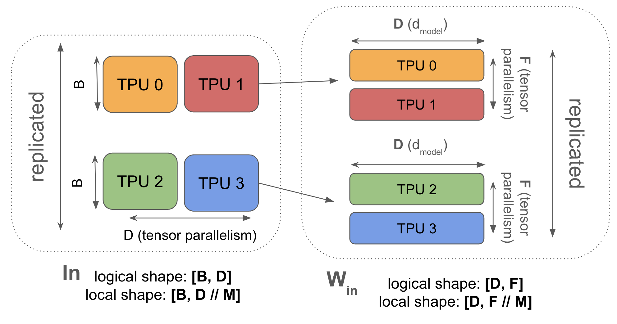
As noted, In[B, DY] *D Win[D, FY] *F Wout[FY, D] -> Out[B, DY] means we have to gather our activations before the first matmul. This is cheaper than ZeRO sharding when the activations are smaller than the weights. This is typically true only with some amount of ZeRO sharding added (which reduces the size of the gather). This is one of the reasons we tend to mix ZeRO sharding and tensor parallelism.
如前所述,In[B, DY] *D Win[D, FY] *F Wout[FY, D] -> Out[B, DY] 意味着我们必须在第一次矩阵乘法之前把激活 gather 起来。当激活比权重更小时,这比 ZeRO 分片更便宜。 这通常只有在额外加了一些 ZeRO 分片(从而缩小 gather 的规模)时才成立。这也是我们倾向于把 ZeRO 分片和张量并行混用的原因之一。
Here's the algorithm for tensor parallelism!
下面是张量并行的算法!
Tensor Parallelism:
张量并行:
Forward pass: need to compute Loss[B]
前向传播: 需要计算 Loss[B]
- In[B, D] = AllGather(In[B, DY]) (on critical path)
- Tmp[B, FY] = In[B, D] *D Win[D, FY] (not sharded along contracting, so no comms)
- Out[B, D] {UY} = Tmp[B, FY] *F Wout[FY, D]
- Out[B, DY] = ReduceScatter(Out[B, D] {UY}) (on critical path)
- Loss[B] = …
- In[B, D] = AllGather(In[B, DY]) (在关键路径上)
- Tmp[B, FY] = In[B, D] *D Win[D, FY] (不沿收缩维分片,所以没有通信)
- Out[B, D] {UY} = Tmp[B, FY] *F Wout[FY, D]
- Out[B, DY] = ReduceScatter(Out[B, D] {UY}) (在关键路径上)
- Loss[B] = …
Backward pass: need to compute dWout[FY, D], dWin[D, FY]
反向传播: 需要计算 dWout[FY, D]、dWin[D, FY]
- dOut[B, DY] = …
- dOut[B, D] = AllGather(dOut[B, DY]) (on critical path)
- dWout[FY, D] = Tmp[B, FY] *B dOut[B, D]
- dTmp[B, FY] = dOut[B, D] *D Wout[FY, D] (can throw away dOut[B, D] here)
- In[B, D] = AllGather(In[B, DY]) (this can be skipped by sharing with (1) from the forward pass)
- dWin[D, FY] = In[B, D] *B dTmp[B, FY]
- dIn[B, D] {UY} = dTmp[B, FY] *F Win[D, FY] (needed for previous layers)
- dIn[B, DY] = ReduceScatter(dIn[B, D] {UY}) (on critical path)
- dOut[B, DY] = …
- dOut[B, D] = AllGather(dOut[B, DY]) (在关键路径上)
- dWout[FY, D] = Tmp[B, FY] *B dOut[B, D]
- dTmp[B, FY] = dOut[B, D] *D Wout[FY, D] (这里可以把 dOut[B, D] 丢掉)
- In[B, D] = AllGather(In[B, DY]) (这可以和前向传播的第 (1) 步共享,从而跳过)
- dWin[D, FY] = In[B, D] *B dTmp[B, FY]
- dIn[B, D] {UY} = dTmp[B, FY] *F Win[D, FY] (前面几层需要用到)
- dIn[B, DY] = ReduceScatter(dIn[B, D] {UY}) (在关键路径上)
One nice thing about tensor parallelism is that it interacts nicely with the two matrices in our Transformer forward pass. Naively, we would do an AllReduce after each of the two matrices. But here we first do In[B, DY] * Win[D, FY] -> Tmp[B, FY] and then Tmp[B, FY] * Wout[FY, D] -> Out[B, DY]. This means we AllGather In at the beginning, and ReduceScatter Out at the end, rather than doing an AllReduce.
张量并行的好处之一是它能和 Transformer 前向传播中的两个矩阵很好地配合。天真做法是在这两个矩阵之后各做一次 AllReduce。但这里我们先后做 In[B, DY] * Win[D, FY] -> Tmp[B, FY],再做 Tmp[B, FY] * Wout[FY, D] -> Out[B, DY]。这意味着我们在开头 AllGather In、在末尾 ReduceScatter Out,而不是做 AllReduce。
How costly is this? Let’s only model the forward pass - the backwards pass is just the transpose of each operation here. In 1D tensor parallelism we AllGather the activations before the first matmul, and ReduceScatter them after the second, sending two bytes at a time (bf16). Let’s figure out when we’re bottlenecked by communication.
这有多贵? 我们只对前向传播建模——反向传播在这里只是每个操作的转置。在 1D 张量并行中,我们在第一次矩阵乘法前 AllGather 激活,在第二次之后 ReduceScatter 激活,每次传两个字节(bf16)。我们来看看什么时候会被通信卡住。
$$\begin{align} T_\text{math} & = \frac{4 \cdot B \cdot D \cdot F}{Y \cdot C} \\ T_\text{comms} & = \frac{2 \cdot 2 \cdot (B \cdot D)}{W_\text{ici}}\\ \textnormal{T} & \approx \max \left(\frac{4 \cdot B \cdot D \cdot F}{Y \cdot C}, \frac{2 \cdot 2 \cdot (B \cdot D)}{W_\text{ici}}\right) \end{align}$$
Noting that we want compute cost to be greater than comms cost, we get:
注意到我们希望计算开销大于通信开销,于是得到:
$$\begin{align} \frac{4 \cdot B \cdot D \cdot F}{Y \cdot C} > \frac{2 \cdot 2 \cdot (B \cdot D)}{W_\text{ici}} \end{align}$$
$$\begin{align} \frac{F}{Y \cdot C} > \frac{1}{W_\text{ici}} \end{align}$$
$$\begin{align} F > Y \cdot \frac{C}{W_\text{ici}} \end{align}$$
Thus for instance, for TPUv5p, $C / W_{ici} = 2550$ in bf16, so we can only do tensor parallelism up to $Y < F / 2550$. When we have multiple ICI axes, our $T_\text{comms}$ is reduced by a factor of $M_Y$, so we get $Y < M_Y \cdot F / 2550$.
举例来说,对 TPUv5p,在 bf16 下 $C / W_{ici} = 2550$,所以张量并行最多只能做到 $Y < F / 2550$。当我们有多条 ICI 轴时,$T_\text{comms}$ 会缩小 $M_Y$ 倍,于是得到 $Y < M_Y \cdot F / 2550$。
Takeaway: Tensor Parallelism becomes communication bound when $Y > M_Y \cdot F / 2550$. For most models this is between 8 and 16-way tensor parallelism.
结论: 当 $Y > M_Y \cdot F / 2550$ 时张量并行变成通信受限。对大多数模型来说,这落在 8 到 16 路张量并行之间。
Note that this doesn’t depend on the precision of the computation, since e.g. for int8, on TPUv5p, $$C_\text{int8} / W_{ici}$$ is $$5100$$ instead of $$2550$$ but the comms volume is also halved, so the two factors of two cancel.
注意,这与计算的精度无关:例如对 int8,在 TPUv5p 上 $$C_\text{int8} / W_{ici}$$ 是 $$5100$$ 而不是 $$2550$$,但通信量也减半,于是这两个因子 2 正好抵消。
Let’s think about some examples:
我们来看几个例子:
- On TPUv5p with LLaMA 3-70B with $$D = 8192,$$ $$F \approx 30,000$$, we can comfortably do 8-way tensor parallelism, but will be communication bound on 16 way tensor parallelism. The required F for 8-way model sharding is 20k.
- 在 TPUv5p 上跑 LLaMA 3-70B,其中 $$D = 8192,$$ $$F \approx 30,000$$,我们可以轻松做到 8 路张量并行,但 16 路张量并行就会通信受限。8 路模型分片所需的 F 是 20k。
- For Gemma 7B, $$F \approx 50k$$, so we become communication bound with 19-way tensor parallelism. That means we could likely do 16-way and still see good performance.
- 对 Gemma 7B,$$F \approx 50k$$,所以到 19 路张量并行才会通信受限。这意味着我们大概可以做到 16 路,性能依然不错。
Combining FSDP and Tensor Parallelism
组合 FSDP 与张量并行
Syntax: $$\text{In}[B_X, D_Y] \cdot_D W_\text{in}[D_X, F_Y] \cdot_F W_\text{out}[F_Y, D_X] \rightarrow \text{Out}[B_X, D_Y]$$
写法: $$\text{In}[B_X, D_Y] \cdot_D W_\text{in}[D_X, F_Y] \cdot_F W_\text{out}[F_Y, D_X] \rightarrow \text{Out}[B_X, D_Y]$$
The nice thing about FSDP and tensor parallelism is that they can be combined. By sharding Win and Wout along both axes we both save memory and compute. Because we shard B along X, we reduce the size of the model-parallel AllGathers, and because we shard F along Y, we reduce the communication overhead of FSDP. This means a combination of the two can get us to an even lower effective batch size than we saw above.
FSDP 和张量并行的一个好处是它们可以组合。把 Win 和 Wout 沿两条轴同时分片,既能省显存也能省计算。因为我们沿 X 分片 B,模型并行的 AllGather 规模变小了;因为我们沿 Y 分片 F,FSDP 的通信开销也变小了。这意味着把两者组合起来,可以让我们达到比上面更低的等效 batch size。
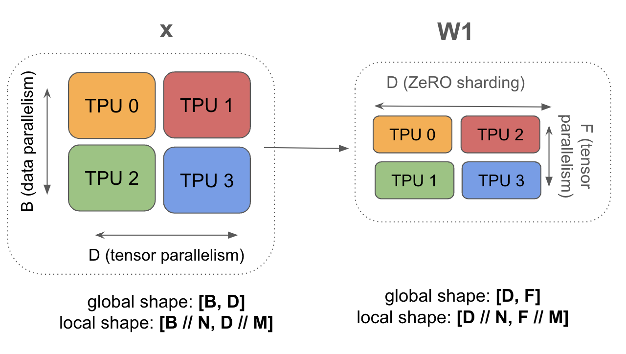
Here's the full algorithm for mixed FSDP + tensor parallelism. While we have a lot of communication, all our AllGathers and ReduceScatters are smaller because we have batch-sharded our activations and tensor sharded our weights much more!
下面是 FSDP + 张量并行混合方案的完整算法。虽然通信很多,但由于我们把激活按 batch 分片、把权重按张量分片得更多,所有 AllGather 和 ReduceScatter 的规模都更小了!
Forward pass: need to compute Loss[B]
前向传播: 需要计算 Loss[B]
- In[BX, D] = AllGatherY(In[BX, DY]) (on critical path)
- Win[D, FY] = AllGatherX(Win[DX, FY]) (can be done ahead of time)
- Tmp[BX, FY] = In[BX, D] *D Win[D, FY]
- Wout[FY, D] = AllGatherX(Wout[FY, DX]) (can be done ahead of time)
- Out[BX, D] {UY} = Tmp[BX, FY] *F Wout[FY, D]
- Out[BX, DY] = ReduceScatterY(Out[BX, D] {UY}) (on critical path)
- Loss[BX] = …
- In[BX, D] = AllGatherY(In[BX, DY]) (在关键路径上)
- Win[D, FY] = AllGatherX(Win[DX, FY]) (可以提前做)
- Tmp[BX, FY] = In[BX, D] *D Win[D, FY]
- Wout[FY, D] = AllGatherX(Wout[FY, DX]) (可以提前做)
- Out[BX, D] {UY} = Tmp[BX, FY] *F Wout[FY, D]
- Out[BX, DY] = ReduceScatterY(Out[BX, D] {UY}) (在关键路径上)
- Loss[BX] = …
Backward pass: need to compute dWout[FY, DX], dWin[DX, FY]
反向传播: 需要计算 dWout[FY, DX]、dWin[DX, FY]
- dOut[BX, DY] = …
- dOut[BX, D] = AllGatherY(dOut[BX, DY]) (on critical path)
- dWout[FY, D] {UX} = Tmp[BX, FY] *B dOut[BX, D]
- dWout[FY, DX] = ReduceScatterX(dWout[FY, D] {UX})
- Wout[FY, D] = AllGatherX(Wout[FY, DX]) (can be done ahead of time)
- dTmp[BX, FY] = dOut[BX, D] *D Wout[FY, D] (can throw away dOut[B, D] here)
- In[BX, D] = AllGatherY(In[BX, DY]) (not on critical path + this can be shared with (2) from the previous layer)
- dWin[D, FY] {UX} = In[BX, D] *B dTmp[BX, FY]
- dWin[DX, FY] = ReduceScatterX(dWin[D, FY] {UX})
- Win[D, FY] = AllGatherX(Win[DX, FY]) (can be done ahead of time)
- dIn[BX, D] {UY} = dTmp[BX, FY] *F Win[D, FY] (needed for previous layers)
- dIn[BX, DY] = ReduceScatterY(dIn[BX, D] {UY}) (on critical path)
- dOut[BX, DY] = …
- dOut[BX, D] = AllGatherY(dOut[BX, DY]) (在关键路径上)
- dWout[FY, D] {UX} = Tmp[BX, FY] *B dOut[BX, D]
- dWout[FY, DX] = ReduceScatterX(dWout[FY, D] {UX})
- Wout[FY, D] = AllGatherX(Wout[FY, DX]) (可以提前做)
- dTmp[BX, FY] = dOut[BX, D] *D Wout[FY, D] (这里可以把 dOut[B, D] 丢掉)
- In[BX, D] = AllGatherY(In[BX, DY]) (不在关键路径上,而且可以和上一层的第 (2) 步共享)
- dWin[D, FY] {UX} = In[BX, D] *B dTmp[BX, FY]
- dWin[DX, FY] = ReduceScatterX(dWin[D, FY] {UX})
- Win[D, FY] = AllGatherX(Win[DX, FY]) (可以提前做)
- dIn[BX, D] {UY} = dTmp[BX, FY] *F Win[D, FY] (前面几层需要用到)
- dIn[BX, DY] = ReduceScatterY(dIn[BX, D] {UY}) (在关键路径上)
What’s the right combination of FSDP and TP? A simple but key maxim is that FSDP moves weights and tensor parallelism moves activations. That means as our batch size shrinks (especially as we do more data parallelism), tensor parallelism becomes cheaper because our activations per-shard are smaller.
FSDP 和 TP 该怎么配比? 有一条简单却关键的准则:FSDP 搬运权重,张量并行搬运激活。这意味着当 batch size 变小时(尤其是当我们做更多数据并行时),张量并行会变得更便宜,因为每个分片上的激活更小了。
- Tensor parallelism performs $$\mathbf{AllGather}_Y([B_X, D_Y])$$ which shrinks as $$X$$ grows.
- FSDP performs $$\mathbf{AllGather}_X([D_X, F_Y])$$ which shrinks as $$Y$$ grows.
- 张量并行执行 $$\mathbf{AllGather}_Y([B_X, D_Y])$$,它随 $$X$$ 增大而变小。
- FSDP 执行 $$\mathbf{AllGather}_X([D_X, F_Y])$$,它随 $$Y$$ 增大而变小。
Thus by combining both we can push our minimum batch size per replica down even more. We can calculate the optimal amount of FSDP and TP in the same way as above:
因此,把两者结合起来,我们可以把每个副本所需的最小 batch size 压得更低。我们可以像上面那样计算 FSDP 与 TP 的最优配比:
Let $$X$$ be the number of chips dedicated to FSDP and $$Y$$ be the number of chips dedicated to tensor parallelism. Let $$N$$ be the total number of chips in our slice with $$N=XY$$. Let $$M_X$$ and $$M_Y$$ be the number of mesh axes over which we do FSDP and TP respectively (these should roughly sum to 3). We’ll purely model the forward pass since it has the most communication per FLOP. Then adding up the comms in the algorithm above, we have
设 $$X$$ 为用于 FSDP 的芯片数,$$Y$$ 为用于张量并行的芯片数。设 $$N$$ 为我们整个 slice 的芯片总数,$$N=XY$$。设 $$M_X$$ 和 $$M_Y$$ 分别为做 FSDP 和 TP 的 mesh 轴数(两者大致加起来应为 3)。我们只对前向传播建模,因为它每 FLOP 的通信量最大。把上面算法里的通信量加起来,得到
$$T_\text{FSDP comms}(B, X, Y) = \frac{2\cdot 2\cdot D \cdot F}{Y \cdot W_\text{ici} \cdot M_X}$$
$$T_\text{TP comms}(B, X, Y) = \frac{2 \cdot 2 \cdot B \cdot D}{X \cdot W_\text{ici} \cdot M_Y}$$
And likewise our total FLOPs time is
同样地,我们的总 FLOPs 时间是
$$T_\text{math} = \frac{2\cdot 2 \cdot B \cdot D \cdot F}{N \cdot C}.$$
To simplify the analysis, we make two assumptions: first, we allow $X$ and $Y$ to take on non-integer values (as long as they are positive and satisfy $XY=N$); second, we assume that we can fully overlap comms on the $X$ and $Y$ axis with each other. Under the second assumption, the total comms time is
为简化分析,我们做两个假设:第一,允许 $X$ 和 $Y$ 取非整数值(只要为正且满足 $XY=N$);第二,假设 X 轴和 Y 轴上的通信可以完全相互重叠。在第二个假设下,总通信时间是
$$T_\text{comms} = \max\left(T_\text{FSDP comms}, T_\text{TP comms}\right)$$
Before we ask under what conditions we’ll be compute-bound, let’s find the optimal values for $X$ and $Y$ to minimize our total communication. Since our FLOPs is independent of $X$ and $Y$, the optimal settings are those that simply minimize comms. To do this, let’s write $T_\text{comms}$ above in terms of $X$ and $N$ (which is held fixed, as it’s the number of chips in our system) rather than $X$ and $Y$:
在问「什么条件下我们才计算受限」之前,先来找让总通信最小的 $X$ 和 $Y$ 最优值。由于我们的 FLOPs 与 $X$、$Y$ 无关,最优设置就是让通信最小的设置。为此,我们把上面的 $T_\text{comms}$ 用 $X$ 和 $N$($N$ 固定,因为它是系统里的芯片数)而不是 $X$ 和 $Y$ 来表示:
$$T_\text{comms} (X) = \frac{4D}{W_\text{ici}} \max\left(\frac{F \cdot X}{N \cdot M_X}, \frac{B}{X \cdot M_Y}\right)$$
Because $T_\text{FSDP comms}$ is monotonically increasing in $X$, and $T_\text{TP comms}$ is monotonically decreasing in $X$, the maximum must be minimized when $T_\text{FSDP comms} = T_\text{TP comms}$, which occurs when
由于 $T_\text{FSDP comms}$ 随 $X$ 单调递增,而 $T_\text{TP comms}$ 随 $X$ 单调递减,最大值一定在 $T_\text{FSDP comms} = T_\text{TP comms}$ 时取到最小,也就是当
$$\begin{align*} \frac{FX_{opt}}{M_X} = \frac{BN}{X_{opt} M_Y} \rightarrow \\ X_{opt} = \sqrt{\frac{B}{F} \frac{M_X}{M_Y} N} \end{align*}$$
This is super useful! This tells us, for a given $B$, $F$, and $N$, what amount of FSDP is optimal. Let’s get a sense of scale. Plugging in realistic values, namely $N = 64$ (corresponding to a 4x4x4 array of chips), $B=48,000$, $F=32768$, gives roughly $X\approx 13.9$. So we would choose $X$ to be 16 and $Y$ to be 4, close to our calculated optimum.
这非常有用!它告诉我们,在给定 $B$、$F$、$N$ 时,多少 FSDP 是最优的。来找个量级感。代入现实中的数值,即 $N = 64$(对应 4x4x4 的芯片阵列)、$B=48,000$、$F=32768$,得到大约 $X\approx 13.9$。所以我们会取 $X$ 为 16、$Y$ 为 4,接近算出的最优值。
Takeaway: in general, during training, the optimal amount of FSDP is $$X_{opt} = \sqrt{\frac{B}{F} \frac{M_X}{M_Y} N}$$.
结论: 一般来说,训练时最优的 FSDP 用量是 $$X_{opt} = \sqrt{\frac{B}{F} \frac{M_X}{M_Y} N}$$。
Now let’s return to the question we’ve been asking of all our parallelism strategies: under what conditions will we be compute-bound? Since we can overlap FLOPs and comms, we are compute-bound when
现在回到我们对所有并行策略都问过的问题:在什么条件下我们会是计算受限? 既然 FLOPs 和通信可以重叠,那么当
$$\max\left(T_\text{FSDP comms}, T_\text{TP comms}\right) < T_\text{math}$$
By letting $\alpha \equiv C / W_\text{ici}$, the ICI arithmetic intensity, we can simplify:
令 $\alpha \equiv C / W_\text{ici}$,即 ICI 算术强度,可以化简为:
$$\max\left(\frac{F}{Y \cdot M_X}, \frac{B}{X \cdot M_Y}\right) < \frac{B \cdot F}{N \cdot \alpha}$$
Since we calculated $X_{opt}$ to make the LHS maximum equal, we can just plug it into either side (noting that $Y_{opt} = N/X_{opt}$), i.e.
由于我们算出的 $X_{opt}$ 会让左边两项的最大值相等,把它代进任意一边即可(注意 $Y_{opt} = N/X_{opt}$),即
$$\frac{F}{N \cdot W_\text{ici} \cdot M_X} \sqrt{\frac{B}{F} \frac{M_X}{M_Y} N} < \frac{B \cdot F}{N \cdot C}$$
Further simplifying, we find that
进一步化简,得到
$$ \sqrt{\frac{B\cdot F}{M_X \cdot M_Y \cdot N}} < \frac{B \cdot F}{N \cdot \alpha},$$
where the left-hand-side is proportional to the communication time and the right-hand-side is proportional to the computation time. Note that while the computation time scales linearly with the batch size (as it does regardless of parallelism), the communication time scales as the square root of the batch size. The ratio of the computation to communication time thus also scales as the square root of the batch size:
其中左边正比于通信时间,右边正比于计算时间。注意,计算时间随 batch size 线性增长(无论用哪种并行都是如此),而通信时间按 batch size 的平方根增长。因此计算与通信时间之比也按 batch size 的平方根增长:
$$ \frac{T_\text{math}}{T_\text{comms}} = \frac{\sqrt{BF}\sqrt{M_X M_Y}}{\alpha \sqrt{N}}. $$
To ensure that this ratio is greater than one so we are compute bound, we require
要保证这个比值大于 1(也就是计算受限),我们需要
$$ \frac{B}{N} > \frac{\alpha^2}{M_X M_Y F}$$
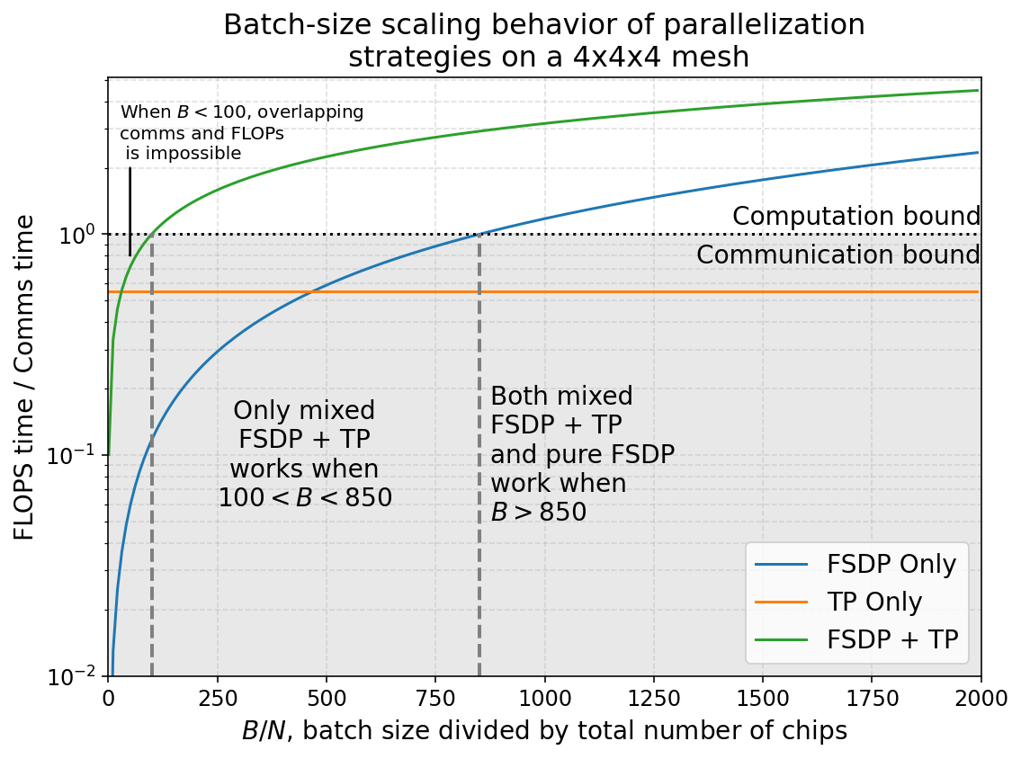
To get approximate numbers, again plug in $F=32,768$, $\alpha=2550$, and $M_X M_Y=2$ (as it must be for a 3D mesh). This gives roughly $B/N > 99$. This roughly wins us a factor of eight compared to the purely data parallel (or FSDP) case, where assuming a 3D mesh we calculate that $B/N$ must exceed about $850$ to be compute bound.
要得到大致数值,再次代入 $F=32,768$、$\alpha=2550$、$M_X M_Y=2$(对 3D mesh 必然如此)。这给出大约 $B/N > 99$。相比纯数据并行(或 FSDP)的情形,这差不多赢了 8 倍——后者在 3D mesh 下我们算出 $B/N$ 必须超过约 $850$ 才能计算受限。
Takeaway: combining tensor parallelism with FSDP allows us to drop to a $B/N$ of $$2550^2 / 2F$$. This lets us handle a batch of as little as 100 per chip, which is roughly a factor of eight smaller than we could achieve with just FSDP.
结论: 把张量并行和 FSDP 组合起来,可以把 $B/N$ 降到 $$2550^2 / 2F$$。这让我们能处理每芯片低至 100 的 batch,大约比只用 FSDP 小 8 倍。
Below we plot the ratio of FLOPs to comms time for mixed FSDP + TP, comparing it both to only tensor parallelism (TP) and only data parallelism (FSDP), on a representative 4x4x4 chip array. While pure FSDP parallelism dominates for very large batch sizes, in the regime where batch size over number of chips is between roughly 100 and 850, a mixed FSDP + TP strategy is required in order to be compute-bound.
下面我们画出混合 FSDP + TP 的 FLOPs 与通信时间之比,并在一个有代表性的 4x4x4 芯片阵列上,把它分别与只用张量并行(TP)和只用数据并行(FSDP)作比较。虽然在非常大的 batch size 下纯 FSDP 占优,但当「batch size / 芯片数」大致落在 100 到 850 之间时,必须用混合 FSDP + TP 策略才能保持计算受限。
Here’s another example of TPU v5p 16x16x16 showing the FLOPs and comms time as a function of batch size for different sharding schemes.
再给一个 TPU v5p 16x16x16 的例子,展示不同分片方案下 FLOPs 和通信时间随 batch size 的变化。
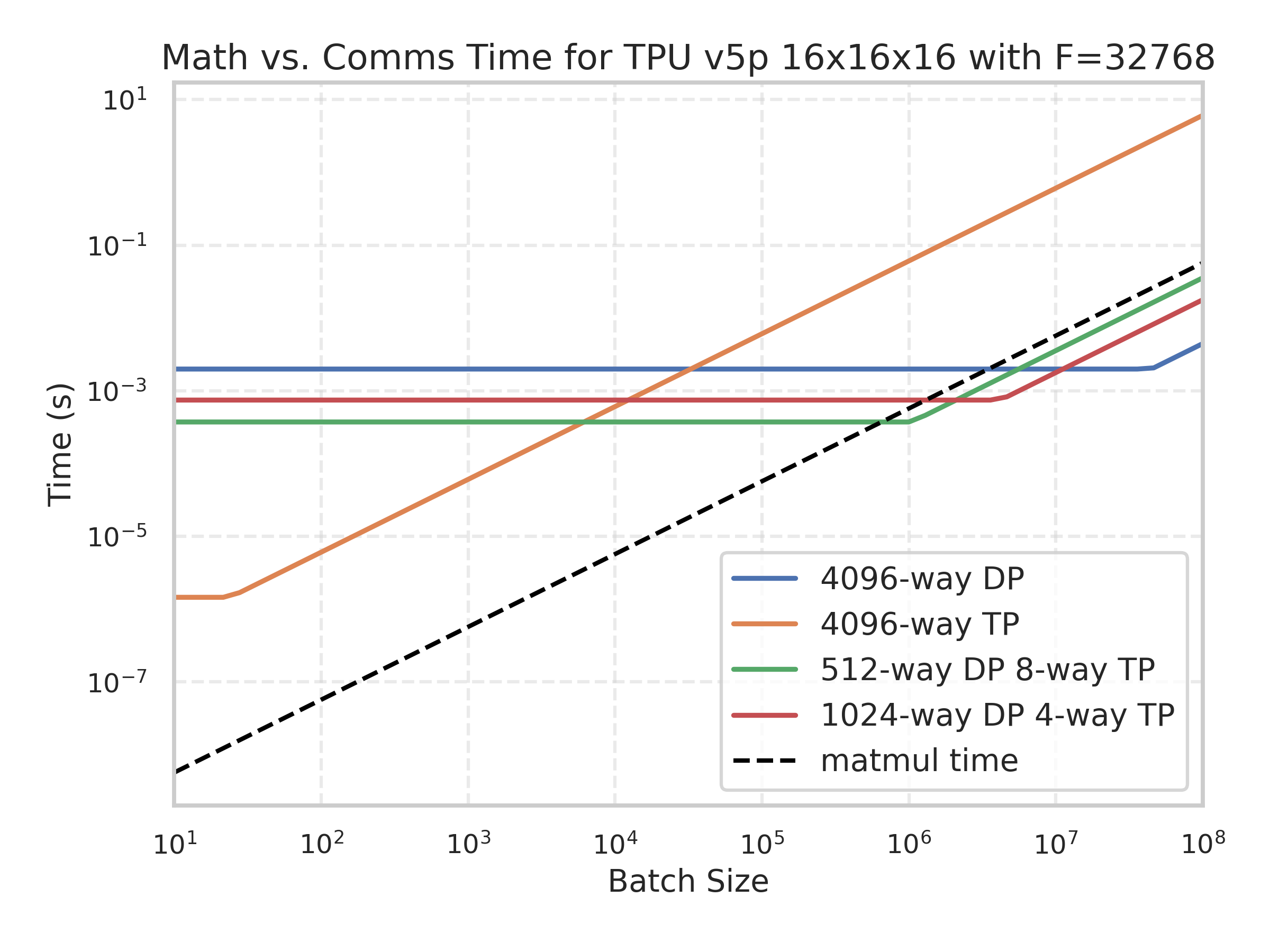
The black curve is the amount of time spent on model FLOPs, meaning any batch size where this is lower than all comms costs is strictly comms bound. You’ll notice the black curve intersects the green curve at about 4e5, as predicted.
黑色曲线是花在模型 FLOPs 上的时间,也就是说,任何让这条曲线低于所有通信开销的 batch size 都严格是通信受限的。你会注意到黑线大约在 4e5 处与绿线相交,和预测一致。
Here’s an interactive animation to play with this, showing the total compute time and communication time for different batch sizes:
这里有一个可以动手玩的交互动画,展示不同 batch size 下的总计算时间和通信时间:
You’ll notice this generally agrees with the above: the best split, FSDP=512 and TP=8, becomes compute-bound above a batch size of about 4e5, while every split with more tensor parallelism stays comms-bound at all batch sizes. Splits with less tensor parallelism need an even larger batch.
你会注意到这和上面的结论基本一致:最优配比 FSDP=512、TP=8 在 batch size 大约超过 4e5 后变成计算受限,而任何张量并行更多的配比在所有 batch size 下都仍是通信受限。张量并行更少的配比则需要更大的 batch。
Pipelining
流水线并行
You’ll probably notice we’ve avoided talking about pipelining at all in the previous sections. Pipelining is a dominant strategy for GPU parallelism that is somewhat less essential on TPUs. Briefly, pipelined training involves splitting the layers of a model across multiple devices and passing the activations between pipeline stages during the forward and backward pass. The algorithm is something like:
你大概已经注意到,前面几节我们完全没提流水线。流水线是 GPU 并行中的一种主导策略,但在 TPU 上没那么不可或缺。简单说,流水线训练把模型的各层切分到多台设备上,并在前向和反向传播中于各流水线阶段之间传递激活。算法大致如下:
- Initialize your data on TPU 0 with your weights sharded across the layer dimension ($W_\text{in}[L_Z, D_X, F_Y]$ for pipelining with FSDP and tensor parallelism).
- Perform the first layer on TPU 0, then copy the resulting activations to TPU 1, and repeat until you get to the last TPU.
- Compute the loss function and its derivative $\partial L / \partial x_L$.
- For the last pipeline stage, compute the derivatives $\partial L / \partial W_L$ and $\partial L / \partial x_{L-1}$, then copy $\partial L / \partial x_{L-1}$ to the previous pipeline stage and repeat until you reach TPU 0.
- 把数据初始化在 TPU 0 上,权重沿层的维度分片(与 FSDP、张量并行一起用时是 $W_\text{in}[L_Z, D_X, F_Y]$)。
- 在 TPU 0 上执行第一层,然后把得到的激活拷贝到 TPU 1,如此重复直到最后一颗 TPU。
- 计算损失函数及其导数 $\partial L / \partial x_L$。
- 对最后一个流水线阶段,计算导数 $\partial L / \partial W_L$ 和 $\partial L / \partial x_{L-1}$,然后把 $\partial L / \partial x_{L-1}$ 拷贝到上一个流水线阶段,重复直到回到 TPU 0。
Here is some (working) Python pseudo-code
下面是一段(能跑通的)Python 伪代码
This pseudocode should run on a Cloud TPU VM. While it’s not very efficient or realistic, it gives you a sense how data is being propagated across devices.
这段伪代码应当能在 Cloud TPU VM 上跑起来。虽然它不是很高效率、也不太写实,但能让你感受到数据是如何在各设备之间传播的。
batch_size = 32
d_model = 128
d_ff = 4 * d_model

num_layers = len(jax.devices())

key = jax.random.PRNGKey(0)

# Pretend each layer is just a single matmul.
x = jax.random.normal(key, (batch_size, d_model))
weights = jax.random.normal(key, (num_layers, d_model, d_model))

def layer_fn(x, weight):
  return x @ weight

# Assume we have num_layers == num_pipeline_stages
intermediates = [x]
for i in range(num_layers):
  x = layer_fn(x, weights[i])
  intermediates.append(x)

  if i != num_layers - 1:
    x = jax.device_put(x, jax.devices()[i+1])

def loss_fn(batch):
  return jnp.mean(batch ** 2)  # make up some fake loss function

loss, dx = jax.value_and_grad(loss_fn)(x)

for i in range(num_layers - 1, -1, -1):
  _, f_vjp = jax.vjp(layer_fn, intermediates[i], weights[i])
  dx, dw = f_vjp(dx)  # compute the jvp dx @ J(L)(x[i], W[i])
  weights[i] = weights[i] - 0.01 * dw  # update our weights

  if i != 0:
    dx = jax.device_put(dx, jax.devices()[i-1])
Why is this a good idea? Pipelining is great for many reasons: it has a low communication cost between pipeline stages, meaning you can train very large models even with low bandwidth interconnects. This is often very useful on GPUs since they are not densely connected by ICI in the way TPUs are.
为什么这是个好主意? 流水线有很多优点:阶段之间的通信开销很低,意味着即使互联带宽很低也能训练非常大的模型。这在 GPU 上常常很有用,因为 GPU 并不像 TPU 那样靠 ICI 密集互联。
Why is this difficult/annoying? You might have noticed in the pseudocode above that TPU 0 is almost always idle! It’s only doing work on the very first and last step of the pipeline. The period of idleness is called a pipeline bubble and is very annoying to deal with. Typically we try to mitigate this first with microbatching, which sends multiple small batches through the pipeline, keeping TPU 0 utilized for at least a larger fraction of the total step time.
为什么它又难又烦? 你可能已经注意到,上面的伪代码里 TPU 0 几乎一直在闲着!它只在流水线的第一步和最后一步干活。这段空闲期被称为 pipeline bubble(流水线气泡),非常难缠。通常我们首先用 microbatching 来缓解:把多个小 batch 送进流水线,让 TPU 0 至少在总步时中占据更大的利用比例。
A second approach is to carefully overlap the forward matmul $W_i @ x_i$, the backward $dx$ matmul $W_i @ \partial L / \partial x_{i+1}$, and the $dW$ matmul $\partial L / \partial x_{i+1} @ x_i$. Since each of these requires some FLOPs, we can overlap them to fully hide the bubble. Here’s a plot from the recent DeepSeek v3 paper[DeepSeek3] showing their “bubble-free” pipeline schedule:
第二种办法是小心地让前向矩阵乘法 $W_i @ x_i$、反向的 $dx$ 矩阵乘法 $W_i @ \partial L / \partial x_{i+1}$,以及 $dW$ 矩阵乘法 $\partial L / \partial x_{i+1} @ x_i$ 相互重叠。由于它们各自都需要一些 FLOPs,我们可以把它们重叠起来,完全把气泡藏掉。下面是最近的 DeepSeek v3 论文[DeepSeek3]里的一张图,展示了他们「无气泡」的流水线调度:

Because it is less critical for TPUs (which have larger interconnected pods), we won’t delve into this as deeply, but it’s a good exercise to understand the key pipelining bottlenecks.
由于它对 TPU 没那么关键(TPU 的互联 pod 更大),我们不会深入展开,但搞清楚流水线的关键瓶颈仍是一个很好的练习。
Scaling Across Pods
跨 Pod 扩展
The largest possible TPU slice is a TPU v5p SuperPod with 8960 chips (and 2240 hosts). When we want to scale beyond this size, we need to cross the Data-Center Networking (DCN) boundary. Each TPU host comes equipped with one or several NICs (Network Interface Cards) that connect the host to other TPU v5p pods over Ethernet. As noted in the TPU Section, each host has about 200Gbps (25GB/s) of full-duplex DCN bandwidth, which is about 6.25GB/s full-duplex (egress) bandwidth per TPU.
可能的最大 TPU slice 是拥有 8960 颗芯片(以及 2240 台主机)的 TPU v5p SuperPod。当我们想扩展到超过这个规模时,就必须跨越数据中心网络(DCN)边界。每台 TPU 主机都配有一块或几块 NIC(网络接口卡),通过以太网把主机连接到其他 TPU v5p pod。如 TPU 一节所述,每台主机约有 200Gbps(25GB/s)的全双工 DCN 带宽,折算到每颗 TPU 大约是 6.25GB/s 的全双工(出方向)带宽。
Typically, when scaling beyond a single pod, we do some form of model parallelism or FSDP within the ICI domain, and then pure data parallelism across multiple pods. Let $N$ be the number of TPUs we want to scale to and $M$ be the number of TPUs per ICI-connected slice. To do an AllReduce over DCN, we can do a ring-reduction over the set of pods, giving us (in the backward pass):
通常,当扩展到单个 pod 之上时,我们在 ICI 域内做某种模型并行或 FSDP,然后在多个 pod 之间做纯数据并行。设 $N$ 为我们想扩展到的 TPU 总数,$M$ 为每个 ICI 互联 slice 中的 TPU 数。要在 DCN 上做 AllReduce,我们可以在一组 pod 上做 ring-reduction,于是(在反向传播中)有:
$$T_\text{math} = \frac{2 \cdot 2 \cdot 2 \cdot BDF}{N \cdot C}$$
$$T_\text{comms} = \frac{2 \cdot 2 \cdot 2 \cdot DF}{M \cdot W_\text{dcn}}$$
The comms bandwidth scales with $M$, since unlike ICI the total bandwidth grows as we grow our ICI domain and acquire more NICs. Simplifying, we find that $T_\text{math} > T_\text{comms}$ when
通信带宽随 $M$ 增长,因为与 ICI 不同,随着 ICI 域扩大、我们获得更多 NIC,总带宽也会增长。化简后,我们发现 $T_\text{math} > T_\text{comms}$ 当
$$\frac{B}{\text{slice}} > \frac{C}{W_\text{dcn}}$$
For TPU v5p, the $\frac{C}{W_\text{dcn}}$ is about 4.59e14 / 6.25e9 = 73,440. This tells us that to efficiently scale over DCN, there is a minimum batch size per ICI domain needed to egress each node.
对 TPU v5p,$\frac{C}{W_\text{dcn}}$ 约为 4.59e14 / 6.25e9 = 73,440。这告诉我们,要想在 DCN 上高效扩展,每个 ICI 域存在一个最小 batch size,才能喂饱每个节点的出向带宽。
How much of a problem is this? To take a specific example, say we want to train LLaMA-3 70B on TPU v5p with a BS of 2M tokens. LLaMA-3 70B has $F\approx 30,000$. From the above sections, we know the following:
这有多大问题? 举个具体例子,假设我们要在 TPU v5p 上用 2M token 的 BS 训练 LLaMA-3 70B。LLaMA-3 70B 有 $F\approx 30,000$。从前面几节我们知道:
- We can do Tensor Parallelism up to $Y = M_Y \cdot F / 2550 \approx 11 \cdot M_Y$.
- We can do FSDP so long as $B / N > 2550 / M_X$. That means if we want to train with BS=2M and 3 axes of data parallelism, we’d at most be able to use $\approx 2400$ chips, roughly a quarter of a TPU v5p pod.
- When we combine FSDP + Tensor Parallelism, become comms-bound when we have $B / N < 2550^2 / (2 \cdot 30000) = 108$, so this lets us scale to roughly 18k chips! However, the maximum size of a TPU v5p pod is 8k chips, so beyond that we have to use DCN.
- 张量并行最多可以做到 $Y = M_Y \cdot F / 2550 \approx 11 \cdot M_Y$。
- 只要 $B / N > 2550 / M_X$ 就可以做 FSDP。这意味着如果我们要用 BS=2M、3 条数据并行轴来训练,最多只能用 $\approx 2400$ 颗芯片,大约是 TPU v5p pod 的四分之一。
- 当把 FSDP + 张量并行组合起来时,$B / N < 2550^2 / (2 \cdot 30000) = 108$ 才会通信受限,所以这能让我们扩展到约 18k 颗芯片!不过 TPU v5p pod 的最大规模是 8k 颗芯片,再往上就必须用 DCN 了。
The TLDR is that we have a nice recipe for training with BS=1M, using roughly X (FSDP) = 1024 and Y (TP) = 8, but with BS=2M we need to use DCN. As noted above, we have a DCN arithmetic intensity of $\text{73,440}$, so we just need to make sure our batch size per ICI domain is greater than this. This is trivial for us, since with 2 pods we’d have a per-pod BS of 1M, and a per TPU batch size of 111, which is great (maybe cutting it a bit close, but theoretically sound).
简单说,BS=1M 时我们有一个漂亮的配方:大致 X(FSDP)= 1024、Y(TP)= 8;但 BS=2M 时就得用 DCN 了。如上面所说,DCN 的算术强度是 $\text{73,440}$,所以我们只需保证每个 ICI 域的 batch size 大于它。这对我们来说轻而易举:用 2 个 pod 时每 pod 的 BS 是 1M,每颗 TPU 的 batch size 是 111,非常好(可能有点贴边,但理论上站得住)。
Takeaway: Scaling across multiple TPU pods is fairly straightforward using pure data parallelism so long as our per-pod batch size is at least 73k tokens.
结论: 只要每个 pod 的 batch size 至少有 73k 个 token,用纯数据并行跨多个 TPU pod 扩展就相当直接。
Takeaways from LLM Training on TPUs
TPU 上 LLM 训练的要点总结
- Increasing parallelism or reducing batch size both tend to make us more communication-bound because they reduce the amount of compute performed per chip.
- 增加并行度或减小 batch size 都倾向于让我们更受通信限制,因为它们都减少了每颗芯片上执行的计算量。
- Up to a reasonable context length (~32k) we can get away with modeling a Transformer as a stack of MLP blocks and define each of several parallelism schemes by how they shard the two/three main matmuls per layer.
- 在合理的上下文长度(约 32k)以内,把 Transformer 建模成一摞 MLP 块是够用的,并可以按每种并行方案如何分片每层那两三个主要矩阵乘法来定义它。
- During training there are 4 main parallelism schemes we consider, each of which has its own bandwidth and compute requirements (data parallelism, FSDP, tensor parallelism, and mixed FSDP + tensor parallelism).
- 训练时我们考虑 4 种主要的并行方案,每种都有自己的带宽与计算需求(数据并行、FSDP、张量并行、以及 FSDP + 张量并行混合)。
| Strategy | Description |
|---|---|
| Data Parallelism | Activations are batch sharded, everything else is fully-replicated, we all-reduce gradients during the backward pass. |
| FSDP | Activations, weights, and optimizer are batch sharded, weights are gathered just before use, gradients are reduce-scattered. |
| Tensor Parallelism (aka Megatron, Model) | Activations are sharded along $$d_\text{model}$$, weights are sharded along $$d_{ff}$$, activations are gathered before Win, the result reduce-scattered after Wout. |
| Mixed FSDP + Tensor Parallelism | Both of the above, where FSDP gathers the model sharded weights. |
| 策略 | 描述 |
|---|---|
| 数据并行 | 激活按 batch 分片,其他一切完全复制,在反向传播中对梯度做 all-reduce。 |
| FSDP | 激活、权重、优化器都按 batch 分片,权重在使用前才 gather,梯度做 reduce-scatter。 |
| 张量并行(又名 Megatron、模型并行) | 激活沿 $$d_\text{model}$$ 分片,权重沿 $$d_{ff}$$ 分片,在 Win 之前 gather 激活,在 Wout 之后对结果做 reduce-scatter。 |
| FSDP + 张量并行混合 | 以上两者兼有,其中 FSDP 负责 gather 分片的模型权重。 |
And here are the “formulas” for each method:
下面是每种方法的「公式」:
$$\small \begin{array}{cc} \text{Strategy} & \text{Formula}\\ \hline \text{DP} & \text{In}[B_X, D] \cdot_D W_\text{in}[D, F] \cdot_F W_\text{out}[F, D] \rightarrow \text{Out}[B_X, D] \\ \text{FSDP} & \text{In}[B_X, D] \cdot_D W_\text{in}[D_X, F] \cdot_F W_\text{out}[F, D_X] \rightarrow \text{Out}[B_X, D] \\ \text{TP} & \text{In}[B, D_Y] \cdot_D W_\text{in}[D, F_Y] \cdot_F W_\text{out}[F_Y, D] \rightarrow \text{Out}[B, D_Y] \\ \text{TP + FSDP} & \text{In}[B_X, D_Y] \cdot_D W_\text{in}[D_X, F_Y] \cdot_F W_\text{out}[F_Y, D_X] \rightarrow \text{Out}[B_X, D_Y] \\ \hline \end{array}$$
- Each of these strategies has a limit at which it becomes network/communication bound, based on their per-device compute and comms. Here’s compute and comms per-layer, assuming $$X$$ is FSDP and $$Y$$ is tensor parallelism.
- 每种策略都有一个临界点,超过它就会变成网络 / 通信受限,这取决于其每设备的计算和通信。下面给出每层的计算量和通信量,其中假定 $$X$$ 是 FSDP、$$Y$$ 是张量并行。
$$ \small \begin{array}{ccc} \text{Strategy} & \text{Compute per layer} & \text{Comms per layer} \\ & \text{(ignoring gating einsum)} & \text{(bytes, forward + backward pass)}\\ \hline \text{DP} & 4BDF/X + 8BDF/X & 0 + 8DF \\ \text{FSDP} & 4BDF/X + 8BDF/X & 4DF + 8DF \\ \text{TP} & 4BDF/Y + 8BDF/Y & 4BD + 4BD \\ \text{FSDP + TP} & 4BDF/(XY) + 8BDF/(XY) & (4BD/X + 4DF/Y) + (8BD/X + 8DF/Y) \\ \hline \end{array}$$
- Pure data parallelism is rarely useful because the model and its optimizer state use bytes = 10x parameter count. This means we can rarely fit more than a few billion parameters in memory.
- 纯数据并行很少有用,因为模型及其优化器状态占用的字节数 = 参数量的 10 倍。这意味着我们很少能装下超过几十亿个参数。
- Data parallelism and FSDP become comms bound when the $$\text{batch size per shard} < C / W$$, the arithmetic intensity of the network. For ICI this is 2,550 and for DCN this is about 71,000. This can be increased with more parallel axes.
- 当 $$\text{每分片 batch size} < C / W$$(网络的算术强度)时,数据并行和 FSDP 会变成通信受限。对 ICI 这个值是 2,550,对 DCN 约为 71,000。用更多并行轴可以把它抬高。
- Tensor parallelism becomes comms bound when $$\lvert Y\rvert > F / 2550$$. This is around 8-16 way for most models. This is independent of the batch size.
- 当 $$\lvert Y\rvert > F / 2550$$ 时张量并行变成通信受限。对大多数模型这大约是 8–16 路。 它与 batch size 无关。
- Mixed FSDP + tensor parallelism allows us to drop the batch size to as low as $$2550^2 / 2F \approx 100$$. This is remarkably low.
- FSDP + 张量并行混合可以把 batch size 降到低至 $$2550^2 / 2F \approx 100$$。这低得惊人。
- Data parallelism across pods requires a minimum batch size per pod of roughly 71,000 before becoming DCN-bound.
- 跨 pod 的数据并行需要每个 pod 的 batch size 至少约 71,000,才不会变成 DCN 受限。
- Basically, if your batch sizes are big or your model is small, things are simple. You can either do data parallelism or FSDP + data parallelism across DCN. The middle section is where things get interesting.
- 基本上,如果你的 batch size 很大、或者模型很小,事情就很简单:要么做数据并行,要么跨 DCN 做 FSDP + 数据并行。中间的区间才是有意思的地方。
Some Problems to Work
一些练习题
Let’s use LLaMA-2 13B as a basic model for this section. Here are the model details:
本节我们用 LLaMA-2 13B 作为基础模型。模型细节如下:
| hyperparam | value |
|---|---|
| L | 40 |
| D | 5,120 |
| F | 13824 |
| N | 40 |
| K | 40 |
| H | 128 |
| V | 32,000 |
| 超参数 | 取值 |
|---|---|
| L | 40 |
| D | 5,120 |
| F | 13824 |
| N | 40 |
| K | 40 |
| H | 128 |
| V | 32,000 |
LLaMA-2 has separate embedding and output matrices and a gated MLP block.
LLaMA-2 有独立的 embedding 矩阵和输出矩阵,以及一个 gated MLP 块。
Question 1: How many parameters does LLaMA-2 13B have (I know that’s silly but do the math)? Note that, as in Transformer Math, LLaMA-3 has 3 big FFW matrices, two up-projection and one down-projection. We ignored the two “gating” einsum matrices in this section, but they behave the same as Win in this section.
问题 1: LLaMA-2 13B 有多少参数(我知道这听起来很傻,但还是算一下)?注意,如Transformer 数学中所述,LLaMA-3 有 3 个大 FFW 矩阵,两个 up-projection 和一个 down-projection。本节我们忽略了两个「gating」einsum 矩阵,但它们在本节中的行为与 Win 相同。
Click here for the answer.
点击查看答案。
- FFW parameters: $$3LDF$$ =
8.5e9 - Attention parameters: $$4DNHL$$ =
4.2e9 - Vocabulary parameters: $$2VD$$ =
0.33e9 - Total:
8.5e9 + 4.2e9 + 0.33e9 = 13.0e9, as expected!
- FFW 参数:$$3LDF$$ =
8.5e9 - 注意力参数:$$4DNHL$$ =
4.2e9 - 词表参数:$$2VD$$ =
0.33e9 - 合计:
8.5e9 + 4.2e9 + 0.33e9 = 13.0e9,符合预期!
Question 2: Let’s assume we’re training with BS=16M tokens and using Adam. Ignoring parallelism for a moment, how much total memory is used by the model’s parameters, optimizer state, and activations? Assume we store the parameters in bf16 and the optimizer state in fp32 and checkpoint activations three times per layer (after the three big FFW matmuls).
问题 2: 假设我们用 BS=16M token 训练并使用 Adam。先不看并行,模型参数、优化器状态和激活一共占用多少显存?假设参数用 bf16 存、优化器状态用 fp32 存,并且每层对激活做三次检查点(在三个大 FFW 矩阵乘法之后)。
Click here for the answer.
点击查看答案。
The total memory used for the parameters (bf16) and the two optimizer states (fp32, the first and second moment accumulators) is (2 + 4 + 4) * 13e9 ~ 130GB. The activations after the first two matmuls are shaped $BF$ and after the last one $BD$ (per the Transformer diagram above), so the total memory for bf16 is $2 \cdot L \cdot (BD + 2 * BF) = 2LB \cdot (D + 2F)$ or 2 * 40 * 16e6 * 5,120 * (1 + 2 * 2.7) ~ 4.2e13 = 42TB, since B=16e6. All other activations are more or less negligible.
参数(bf16)和两个优化器状态(fp32,即一阶、二阶矩累加器)占用的总显存是 (2 + 4 + 4) * 13e9 ~ 130GB。前两次矩阵乘法之后的激活形状是 $BF$,最后一次之后是 $BD$(按上面的 Transformer 图),所以 bf16 激活的总显存是 $2 \cdot L \cdot (BD + 2 * BF) = 2LB \cdot (D + 2F)$,即 2 * 40 * 16e6 * 5,120 * (1 + 2 * 2.7) ~ 4.2e13 = 42TB(因为 B=16e6)。其他所有激活基本可以忽略不计。
Question 3: Assume we want to train with 32k sequence length and a total batch size of 3M tokens on a TPUv5p 16x16x16 slice. Assume we want to use bfloat16 weights and a float32 optimizer, as above.
问题 3: 假设我们要在 TPUv5p 16x16x16 slice 上,用 32k 序列长度、总计 3M token 的 batch 训练。假设像上面一样用 bfloat16 权重和 float32 优化器。
- Can we use pure data parallelism? Why or why not?
- Can we use pure FSDP without being comms-bound? Why or why not? With pure FSDP, how much memory will be used per device (assume we do gradient checkpointing only after the 3 big FFW matrices).
- Can we use mixed FSDP + tensor parallelism? Why or why not? If so, what should $X$ and $Y$ be? How much memory will be stored per device? Using only roofline FLOPs estimates and ignoring attention, how long will each training step take at 40% MFU?
- 我们能使用纯数据并行吗?为什么能或不能?
- 我们能使用纯 FSDP 而不受通信限制吗?为什么能或不能?用纯 FSDP 时每设备会占用多少显存(假设只在三个大 FFW 矩阵之后做梯度检查点)。
- 我们能使用 FSDP + 张量并行混合吗?为什么能或不能?如果可以,$X$ 和 $Y$ 应该取多少?每设备会存多少显存?只用 roofline FLOPs 估计并忽略注意力,在 40% MFU 下每一步训练要多久?
Click here for the answer.
点击查看答案。
First, let’s write down some numbers. With 32k sequence length and a 3M batch size, we have a sequence batch size of 96. On a TPU v5p 16x16x16 slice, we have 393TB of HBM.
首先写下一些数字。序列长度 32k、batch size 3M 时,序列 batch size 是 96。一个 TPU v5p 16x16x16 slice 有 393TB 的 HBM。
- We can’t use pure data parallelism, because it replicates the parameters and optimizer states on each chip, which are already around 130GB (from Q2) which is more HBM than we have per-chip (96GB).
- 我们不能用纯数据并行,因为它会在每颗芯片上复制参数和优化器状态,而这已经有约 130GB(来自问题 2),超过了每芯片的 HBM 容量(96GB)。
- Let’s start by looking purely at memory. Replacing BS=16M with 3M in Q2, we get
~7.86e12total checkpoint activations, and with the 1.3e11 optimizer state this brings us to almost exactly 8e12 = 8TB. The TPUv5p slice has393TBof HBM in total, so we are safely under the HBM limit. Next let’s look at whether we’ll be comms or compute-bound. With 4096 chips and 3 axes of parallelism, we can do a minimum batch size of850 * 4096 = 3.48Mtokens. That’s slightly above our 3M batch size. So we’re actually comms-bound, which is sad. So the general answer is no, we cannot do FSDP alone without being comms-bound.
- 先从显存看。把问题 2 里的 BS=16M 换成 3M,得到检查点激活总量约
~7.86e12,再加上 1.3e11 的优化器状态,几乎正好是 8e12 = 8TB。这个 TPUv5p slice 的 HBM 总量是393TB,所以我们远低于 HBM 上限。接着看我们会是通信受限还是计算受限。用 4096 颗芯片、3 条并行轴,我们能支持的最小 batch size 是850 * 4096 = 3.48M个 token,略高于我们的 3M。所以其实我们会通信受限,有点可惜。因此总体答案是:不行,单用 FSDP 无法避免通信受限。
- Now we know our primary concern is being comms-bound, so let’s plug in some numbers. First of all, we know from above that our per-chip batch size with mixed FSDP + tensor parallelism needs to be above $2550^2 / 2F = 235$ here. That means we can in theory do this! Let’s figure out how much of each.
- 现在我们知道主要担心的是通信受限,那就代入一些数字。首先,从上面知道,FSDP + 张量并行混合时每芯片 batch size 需要高于 $2550^2 / 2F = 235$。这意味着理论上我们做得到!我们来算算各自该用多少。
We have the rule $X_{opt} = \sqrt{(B / F) \cdot (M_X / M_Y) \cdot N}$, so here we have sqrt(3e6 * 2 * 4096 / 13824) = 1333, meaning we’ll do roughly 1024 way DP and 4 way TP. Per TPU memory will be as in (2), and step time will just be 6 * 3e6 * 13e9 / (4096 * 4.6e14 * 0.4) = 300ms.
我们有公式 $X_{opt} = \sqrt{(B / F) \cdot (M_X / M_Y) \cdot N}$,这里即 sqrt(3e6 * 2 * 4096 / 13824) = 1333,意味着我们大致会做 1024 路 DP 和 4 路 TP。每颗 TPU 的显存与第 (2) 问相同,步时就是 6 * 3e6 * 13e9 / (4096 * 4.6e14 * 0.4) = 300ms。
That’s it for Part 5! For Part 6, which applies this content to real LLaMA models, click here!
第 5 篇到此结束!第 6 篇会把这些内容套用到真实的 LLaMA 模型上,点这里!
Appendix
附录
Appendix A: Deriving the backward pass comms
附录 A:推导反向传播的通信量
Above, we simplified the Transformer layer forward pass as Out[B, D] = In[B, D] *D Win[D, F] *F Wout[F, D]. How do we derive the comms necessary for the backwards pass?
上面我们把 Transformer 层的前向传播简化成 Out[B, D] = In[B, D] *D Win[D, F] *F Wout[F, D]。那么我们如何推导反向传播所需的通信量?
This follows fairly naturally from the rule in the previous section for a single matmul Y = X * A:
这可以很自然地从上一节关于单次矩阵乘法 Y = X * A 的规则推出:
$$\frac{dL}{dA} = \frac{dL}{dY}\frac{dY}{dA} = X^T \left(\frac{dL}{dY}\right)$$
$$\frac{dL}{dX} = \frac{dL}{dY}\frac{dY}{dX} = \left(\frac{dL}{dY}\right) A^T$$
Using this, we get the following formulas (letting Tmp[B, F] stand for In[B, D] * Win[D, F]):
利用它,我们得到下面的公式(用 Tmp[B, F] 表示 In[B, D] * Win[D, F]):
- dWout[F, D] = Tmp[B, F] *B dOut[B, D]
- dTmp[B, F] = dOut[B, D] *D Wout[F, D]
- dWin[D, F] = In[B, D] *B dTmp[B, F]
- dIn[B, D] = dTmp[B, F] *F Win[D, F]
Note that these formulas are mathematical statements, with no mention of sharding. The job of the backwards pass is to compute these four quantities. So to figure out the comms necessary, we just take the shardings of all the quantities which are to be matmulled in the four equations above (Tmp, dOut, Wout, Win), which are specified by our parallelization scheme, and use the rules of sharded matmuls to figure out what comms we have to do. Note that dOut is sharded in the same way as Out.
注意,这些公式都是数学陈述,完全没提分片。反向传播的任务就是计算这四个量。所以,要弄清需要多少通信,我们只需取上面四个等式里所有参与矩阵乘法的量(Tmp、dOut、Wout、Win)的分片方式(由我们的并行方案指定),再用分片矩阵乘法的规则算出必须做哪些通信。注意 dOut 的分片方式和 Out 相同。
讨论
用 GitHub 账号留言;评论保存在公开仓库chengshu-blog-discussions的 Discussions 里。也可通过 RSS 订阅后续文章。