如何扩展你的模型(3):分片矩阵与分片矩阵乘法
中英对照第 3 篇:用「分片矩阵乘法」这把钥匙打开多设备并行——各种分片方式(replicated / sharded / 混合)下 AllGather、ReduceScatter、AllReduce 的通信代价是怎么算出来的。左栏原文,右栏译文。
本篇属于系列 如何扩展你的模型(How To Scale Your Model) · 第 3 篇
原文:How To Scale Your Model(Google DeepMind,作者 Jacob Austin、Sholto Douglas、Roy Frostig、Anselm Levskaya、Charlie Chen、Sharad Vikram、Federico Lebron、Peter Choy、Vinay Ramasesh、Albert Webson、Reiner Pope)。
本站是中英对照排版:左栏是英文原文,右栏是对应的中文译文。不好直译的术语(roofline、strong scaling、ICI、MXU、KV cache、FSDP、TP 等)保留英文写法;原文配图全部保留。
本文是系列《如何扩展你的模型(How To Scale Your Model)》的第 3 篇,共 13 篇。系列目录。
原文以 MIT 许可证发布,版权归 Google LLC;本译文仅作学习交流之用,如有错漏以原文为准。
Partitioning Notation and Collective Operations
分片记号与集合通信
When we train an LLM on ten thousand TPUs or GPUs, we’re still doing abstractly the same computation as when we’re training on one. The difference is that our arrays don’t fit in the HBM of a single TPU/GPU, so we have to split them. (It’s worth noting that we may also choose to parallelize for speed. Even if we could fit on a smaller number of chips, scaling to more simply gives us more FLOPs/s. During inference, for instance, we can sometimes fit on smaller topologies but choose to scale to larger ones in order to reduce latency. Likewise, during training we often scale to more chips to reduce the step time.) We call this “sharding” or “partitioning” our arrays. The art of scaling is figuring out how to shard our models so computation remains efficient.
当我们在上万块 TPU 或 GPU 上训练一个 LLM 时,抽象地看,我们做的事和在单块芯片上训练没有区别。差别在于我们的数组装不进单块 TPU/GPU 的 HBM,所以必须把它们切开。(值得一提的是,我们有时也会为了速度而并行:即使放得下,用更多芯片也只是给我们更多 FLOPs/s。比如推理时,我们有时明明能塞进更小的拓扑,却仍然选择扩展,只为了降低延迟;训练时我们也常常用更多芯片来缩短单步耗时。)我们管这件事叫对数组做「分片」(sharding)或「划分」(partitioning)。扩展这门手艺,就是想清楚该怎么切分模型,同时让计算依然高效。
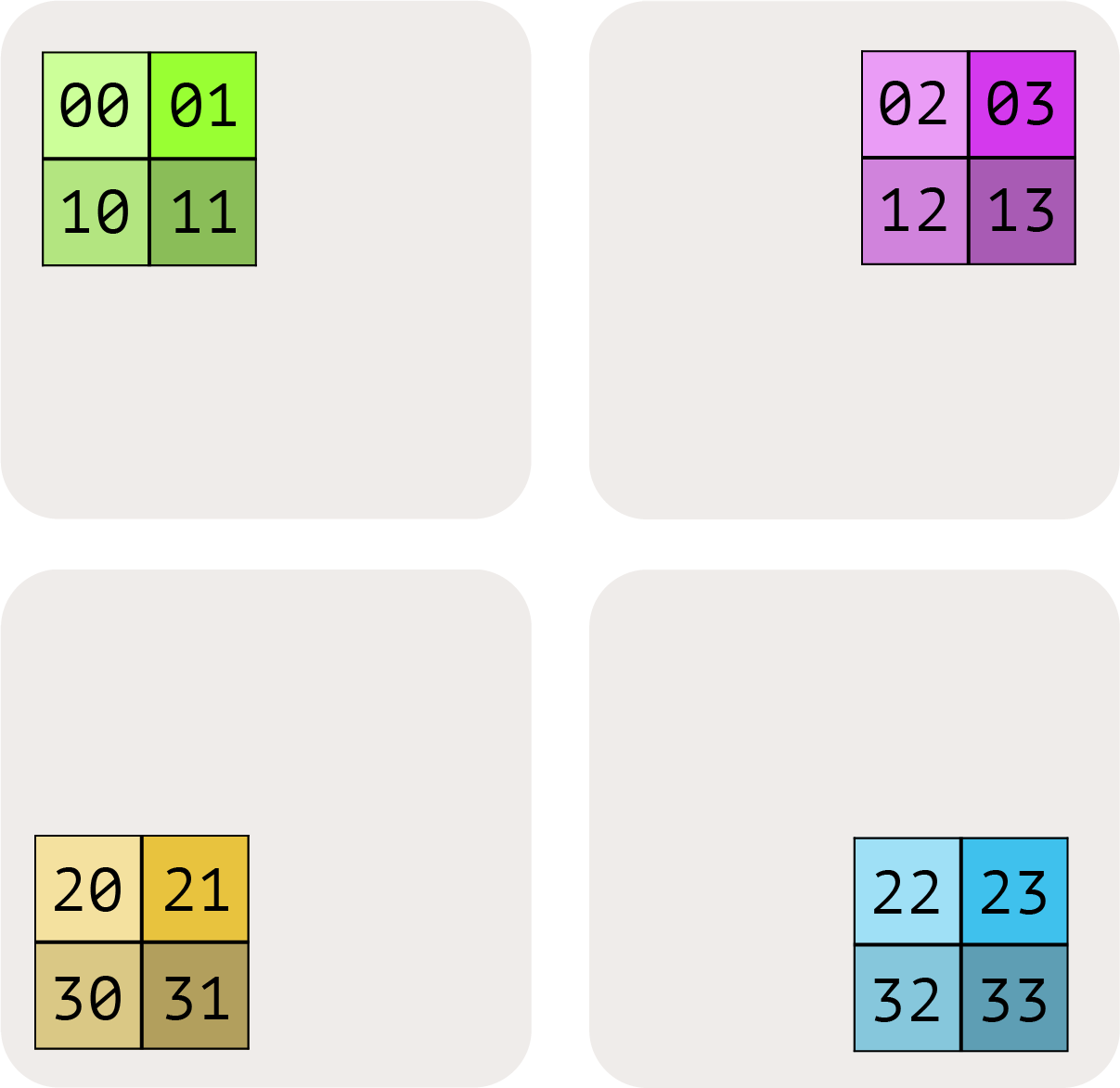
Here’s an example 2D array A sharded across 4 TPUs:
下面是一个 2D 数组 A 被分片到 4 块 TPU 上的例子:
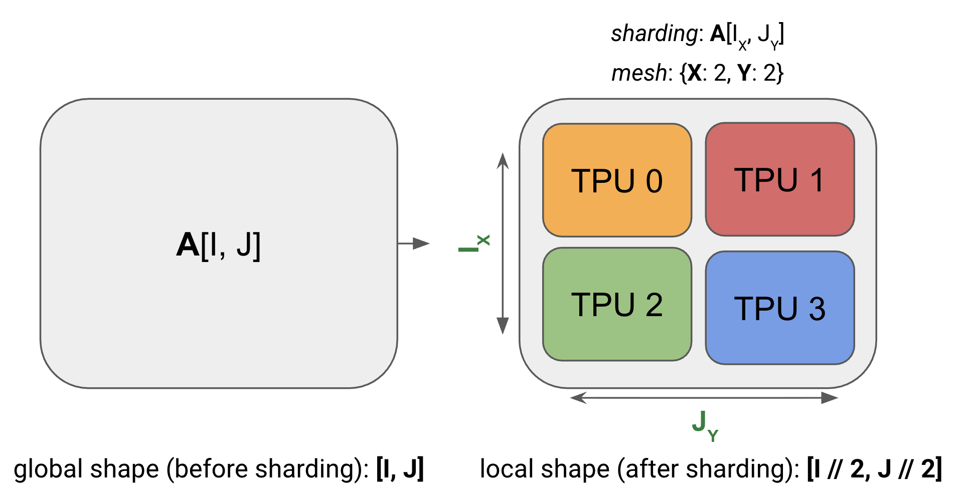
Note how the sharded array still has the same global or logical shape as the unsharded array, say (4, 128), but it also has a device local shape, like (2, 64), which gives us the actual size in bytes that each TPU is holding (in the figure above, each TPU holds ¼ of the total array). Now we’ll generalize this to arbitrary arrays.
注意分片后的数组仍然保有和未分片时相同的全局形状(global / logical shape),比如 (4, 128),但它还有一个设备本地形状(device local shape),比如 (2, 64)——后者决定了每块 TPU 实际持有多少字节(上图中每块 TPU 持有整个数组的 ¼)。接下来我们把它推广到任意数组。
A unified notation for sharding
分片的统一记号
We use a variant of named-axis notation to describe how the tensor is sharded in blocks across the devices: we assume the existence of a 2D or 3D grid of devices called the device mesh where each axis has been given mesh axis names e.g. X, Y, and Z. We can then specify how the matrix data is laid out across the device mesh by describing how each named dimension of the array is partitioned across the physical mesh axes. We call this assignment a sharding.
我们用一套变体的命名轴记号(named-axis notation)来描述张量是如何按块切分到设备上的:先假设存在一个 2D 或 3D 的设备网格,称为设备网格(device mesh),其中每个轴都被赋予一个网格轴名,例如 X、Y、Z。然后我们通过描述数组的每个命名维度如何划分到物理网格轴上,来指定矩阵数据的布局。我们把这个对应关系称为一个分片(sharding)。
Example (the diagram above): For the above diagram, we have:
示例(上图):对上图而言,我们有:
- Mesh: the device mesh above
Mesh(devices=((0, 1), (2, 3)), axis_names=('X', 'Y')), which tells us we have 4 TPUs in a 2x2 grid, with axis names $X$ and $Y$. - Sharding: $A[I_X, J_Y]$, which tells us to shard the first axis, $I$, along the mesh axis $X$, and the second axis, $J$, along the mesh axis $Y$. This sharding tells us that each shard holds $1 / (\lvert X\rvert \cdot \lvert Y\rvert)$ of the array.
- Mesh(网格):上面的设备网格
Mesh(devices=((0, 1), (2, 3)), axis_names=('X', 'Y')),它告诉我们有 4 块 TPU 排成 2x2 的网格,轴名是 $X$ 和 $Y$。 - Sharding(分片):$A[I_X, J_Y]$,它表示把第一个轴 $I$ 沿网格轴 $X$ 分片,把第二个轴 $J$ 沿网格轴 $Y$ 分片。这个分片告诉我们每个分片持有数组的 $1 / (\lvert X\rvert \cdot \lvert Y\rvert)$。
Taken together, we know that the local shape of the array (the size of the shard that an individual device holds) is $(\lvert I\rvert / 2, \lvert J\rvert / 2)$, where $$\lvert I\rvert$$ is the size of A’s first dimension and $$\lvert J\rvert$$ is the size of A’s second dimension.
合起来看,数组的本地形状(单块设备持有的分片大小)是 $(\lvert I\rvert / 2, \lvert J\rvert / 2)$,其中 $$\lvert I\rvert$$ 是 A 第一个维度的大小,$$\lvert J\rvert$$ 是 A 第二个维度的大小。
Pop Quiz [2D sharding across 1 axis]: Consider an array fp32[1024, 4096] with sharding $A[I_{XY}, J]$ and mesh {'X': 8, 'Y': 2}. How much data is held by each device? How much time would it take to load this array from HBM on H100s (assuming 3.4e12 memory bandwidth per chip)?
随堂小测 [跨 1 个轴的 2D 分片]: 考虑一个 fp32[1024, 4096] 的数组,分片为 $A[I_{XY}, J]$,网格 {'X': 8, 'Y': 2}。每块设备持有多少数据?在 H100 上把它从 HBM 加载进来要多久(假设每芯片 3.4e12 的内存带宽)?
Click here for the answer.
点这里看答案。
$A[I_{XY}, J]$ shards the first dimension (I) along both the X and Y hardware axes. In this example, the local shape is $(\lvert I\rvert /(\lvert X\rvert \cdot \lvert Y\rvert), \lvert J\rvert)$. For the given example, the global shape is fp32[1024, 4096], so the local shape is fp32[64, 4096].
$A[I_{XY}, J]$ 把第一个维度(I)同时沿 X 和 Y 两个硬件轴分片。在这个例子里,本地形状是 $(\lvert I\rvert /(\lvert X\rvert \cdot \lvert Y\rvert), \lvert J\rvert)$。给定全局形状 fp32[1024, 4096],本地形状就是 fp32[64, 4096]。
Since each GPU has 4 * 64 * 4096 = 1MiB bytes, this would take about 1e6 / 3.4e12 = 294ns, although likely significantly more due to various overheads since this is so small.
每块 GPU 上是 4 * 64 * 4096 = 1MiB 字节,所以大约要 1e6 / 3.4e12 = 294ns;不过数据这么小,各种开销会让实际耗时明显更长。
Visualizing these shardings: Let’s try to visualize these shardings by looking at a 2D array of data split over 4 devices:
把这些分片画出来: 让我们用一个切成 4 份的 2D 数组来直观看看这些分片:
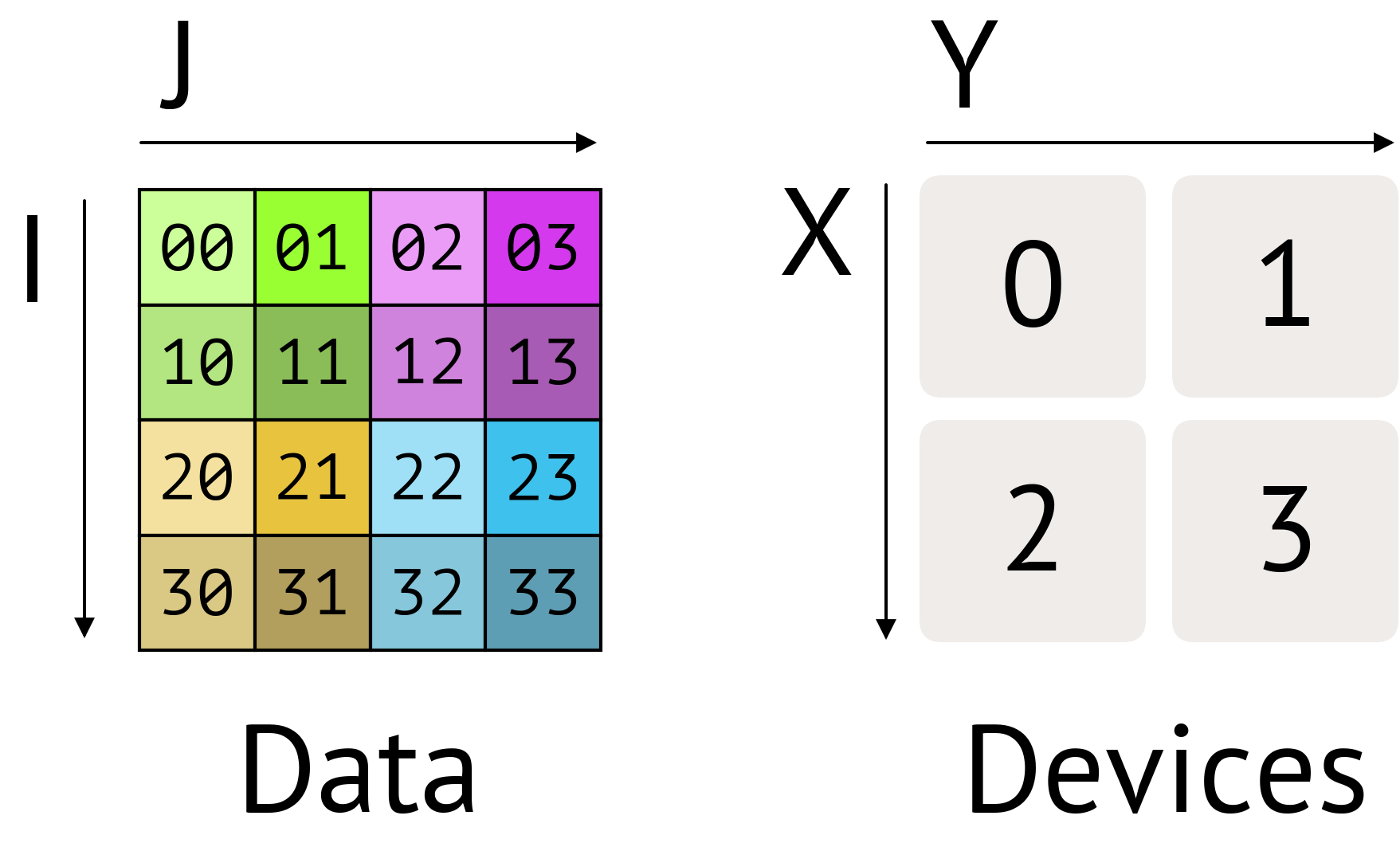
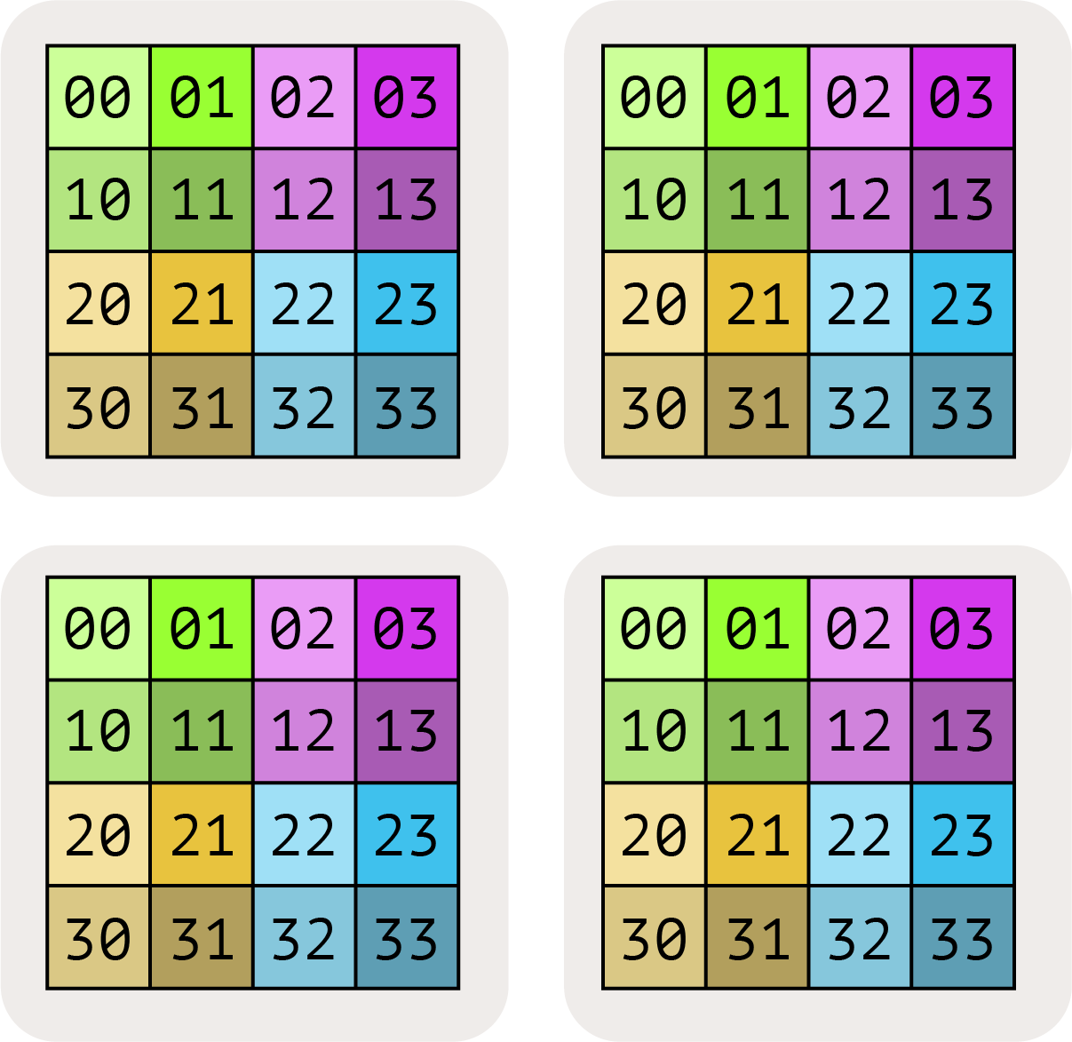
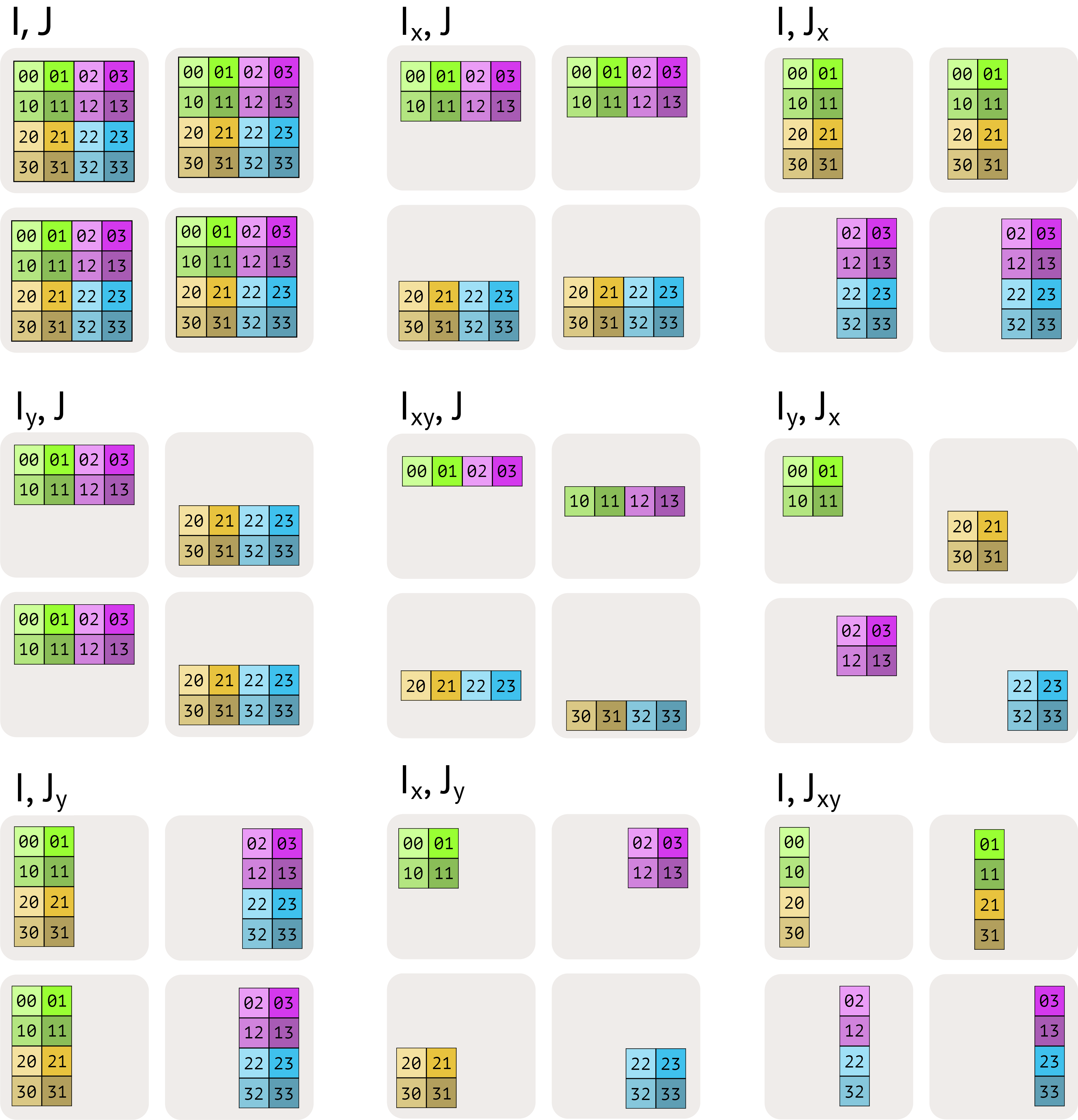
We write the fully-replicated form of the matrix simply as $A[I, J]$ with no sharding assignment. This means that each device contains a full copy of the entire matrix.
我们把矩阵的完全复制(fully-replicated)形式直接写成 $A[I, J]$,不带任何分片标注。这意味着每块设备都持有整个矩阵的一份完整拷贝。
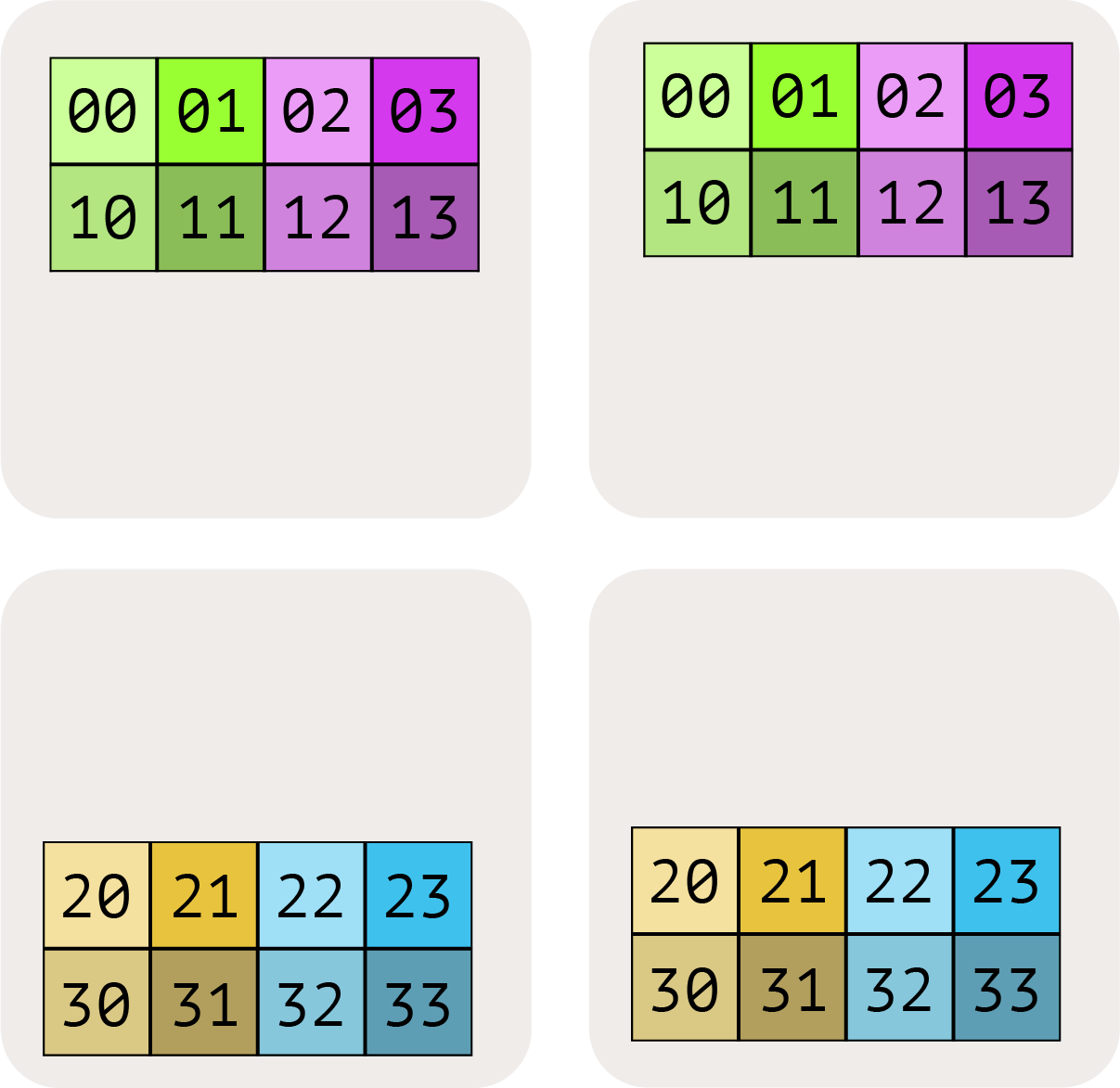
We can indicate that one of these dimensions has been partitioned across a mesh axis with a subscript mesh axis. For instance $A[I_X, J]$ would mean that the I logical axis has been partitioned across the X mesh dimension, but that the J dimension is not partitioned, and the blocks remain partially-replicated across the Y mesh axis.
我们可以用网格轴下标来表示某个维度被划分到了某个网格轴上。例如 $A[I_X, J]$ 表示 I 这个逻辑轴被划分到 X 网格维度上,而 J 维度没有被划分,各块在 Y 网格轴上保持部分复制。
$A[I_X, J_Y]$ means that the I logical axis has been partitioned across the X mesh axis, and that the J dimension has been partitioned across the Y mesh axis.
$A[I_X, J_Y]$ 表示 I 逻辑轴被划分到 X 网格轴上,而 J 维度被划分到 Y 网格轴上,因此每个设备持有数组的 1/4。
We illustrate the other possibilities in the figure below:
下面这张图画出了其余几种可能:
Here $A[I_{XY}, J]$ means that we treat the X and Y mesh axes as a larger flattened dimension and partition the I named axis across all the devices. The order of the multiple mesh-axis subscripts matters, as it specifies the traversal order of the partitioning across the grid.
这里 $A[I_{XY}, J]$ 表示我们把 X 和 Y 两个网格轴视为一个更大的展平维度,把 I 命名轴划分到所有设备上。多个网格轴下标的书写顺序很重要,它指定了划分在网格上的遍历顺序。
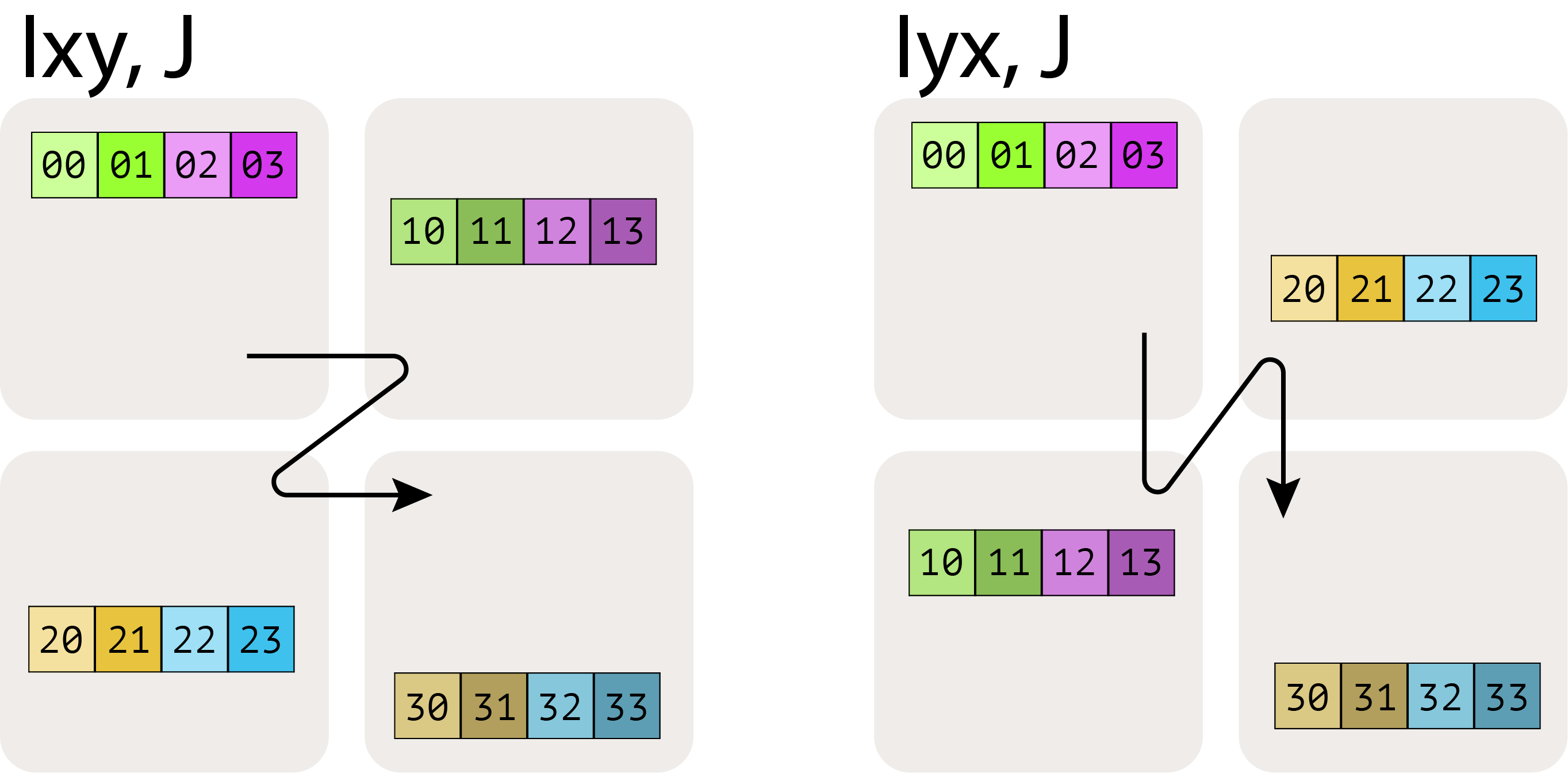
Lastly, note that we cannot have multiple named axes sharded along the same mesh dimension. e.g. $A[I_X, J_X]$ is a nonsensical, forbidden sharding. Once a mesh dimension has been used to shard one dimension of an array, it is in a sense “spent”.
最后要注意,我们不能把多个命名轴分片到同一个网格维度上。例如 $A[I_X, J_X]$ 是无意义、被禁止的分片。一旦某个网格维度被用来分片数组的某个维度,它在某种意义上就「用掉了」。
Pop Quiz: Let A be an array with shape int8[128, 2048], sharding $A[I_{XY}, J]$, and mesh Mesh({'X': 2, 'Y': 8, 'Z': 2}) (so 32 devices total). How much memory does A use per device? How much total memory does A use across all devices?
随堂小测: 设 A 是一个形状为 int8[128, 2048] 的数组,分片为 $A[I_{XY}, J]$,网格为 Mesh({'X': 2, 'Y': 8, 'Z': 2})(共 32 块设备)。A 每块设备占多少内存?A 在所有设备上一共占多少内存?
Click here for the answer.
点这里看答案。
Answer: Our array A is sharded over X and Y and replicated over Z, so per device it has shape int8[128 / (2 * 8), 2048] = int8[8, 2048], with size 8 * 2048 = 16,384 bytes. Because it’s replicated over Z, while within a Z-plane it’s fully sharded over X and Y, there are 2 complete copies of the original array (one per Z-plane). So the total size across all devices is: original array size × Z replicas = 128 * 2048 * 2 = 512 KiB total. Alternatively, we can verify this as: 32 devices × 16,384 bytes per device = 512 KiB total.
答案: 我们的数组 A 在 X 和 Y 上分片、在 Z 上复制,所以每块设备上的形状是 int8[128 / (2 * 8), 2048] = int8[8, 2048],大小是 8 * 2048 = 16,384 字节。由于它在 Z 上被复制,而在每个 Z 平面内部又在 X 和 Y 上完全分片,所以原数组共有 2 份完整拷贝(每个 Z 平面一份)。因此所有设备加起来的总大小是:原数组大小 × Z 份拷贝 = 128 * 2048 * 2 = 512 KiB。换一种算法验证:32 块设备 × 每块 16,384 字节 = 512 KiB。
How do we describe this in code?
用代码怎么描述?
So far we’ve avoided talking about code, but now is a good chance for a sneak peek. JAX uses a named sharding syntax that very closely matches the abstract syntax we describe above. We’ll talk more about this in Section 10, but here’s a quick preview. You can play with this in a Google Colab here and profile the result to see how JAX handles different shardings. This snippet does 3 things:
到目前为止我们一直避开代码,但这里正好可以先偷看一眼。JAX 的命名分片语法和我们上面描述的抽象语法几乎一一对应。我们会在第 10 节里详细讲,这里先给一个预览。你可以在这个 Google Colab 里动手试一试,并 profile 结果,看看 JAX 是怎么处理不同分片的。这段代码做了三件事:
- Creates a jax.Mesh that maps our 8 TPUs into a 4x2 grid with names ‘X’ and ‘Y’ assigned to the two axes.
- Creates matrices A and B where A is sharded along both its dimensions and B is sharded along the output dimension.
- Compiles and performs a simple matrix multiplication that returns a sharded array.
- 创建一个 jax.Mesh,把我们的 8 块 TPU 映射成 4x2 的网格,两个轴分别命名为 ‘X’ 和 ‘Y’。
- 创建矩阵 A 和 B,其中 A 沿两个维度分片,B 沿输出维度分片。
- 编译并执行一次简单的矩阵乘法,返回一个分片数组。
import jax
import jax.numpy as jnp

# Create our mesh! We're running on a TPU v2-8 4x2 slice with names 'X' and 'Y'.
# The Auto axis type tells JAX to let the XLA compiler infer intermediate shardings.
assert len(jax.devices()) == 8
Auto = jax.sharding.AxisType.Auto
mesh = jax.make_mesh(axis_sizes=(4, 2), axis_names=('X', 'Y'), axis_types=(Auto, Auto))

# A little utility function to help define our sharding. A PartitionSpec is our
# sharding (a mapping from axes to names).
def P(*args):
  return jax.NamedSharding(mesh, jax.sharding.PartitionSpec(*args))

# We shard both A and B over the non-contracting dimension and A over the contracting dim.
A = jnp.zeros((8, 2048), dtype=jnp.bfloat16, device=P('X', 'Y'))
B = jnp.zeros((2048, 8192), dtype=jnp.bfloat16, device=P(None, 'Y'))

# We can perform a matmul on these sharded arrays! out_shardings tells us how we want
# the output to be sharded. JAX/XLA handles the rest of the sharding for us.
y = jax.jit(lambda A, B: jnp.einsum('BD,DF->BF', A, B), out_shardings=P('X', 'Y'))(A, B)
The cool thing about JAX is that these arrays behave as if they’re unsharded! B.shape will tell us the global or logical shape (2048, 8192). We have to actually look at B.addressable_shards to see how it’s locally sharded. We can perform operations on these arrays and JAX will attempt to figure out how to broadcast or reshape them to perform the operations. For instance, in the above example, the local shape of A is [2, 1024] and for B is [2048, 4096]. JAX/XLA will automatically add communication across these arrays as necessary to perform the final multiplication.
JAX 最妙的地方在于:这些数组用起来和没分片一样!B.shape 会告诉你全局(逻辑)形状 (2048, 8192)。只有去看 B.addressable_shards,你才能知道它在本地是怎么分片的。我们可以对这些数组做运算,JAX 会试着推断出该如何广播或 reshape 它们来完成运算。比如在上面的例子里,A 的本地形状是 [2, 1024],B 的是 [2048, 4096]。JAX/XLA 会在必要时自动给这些数组加上通信,来完成最终的乘法。
Computation With Sharded Arrays
分片数组上的计算
If you have an array of data that’s distributed across many devices and wish to perform mathematical operations on it, what are the overheads associated with sharding both the data and the computation?
如果你有一个分布到很多设备上的数组,想在它上面做数学运算,那么既分片数据、又分片计算会带来多少开销?
Obviously, this depends on the computation involved.
显然,这取决于具体是什么运算。
- For elementwise operations, there is no overhead for operating on a distributed array.
- When we wish to perform operations across elements resident on many devices, things get complicated. Thankfully, for most machine learning nearly all computation takes place in the form of matrix multiplications, and they are relatively simple to analyze.
- 对逐元素(elementwise)运算来说,在分布式数组上操作没有任何额外开销。
- 当我们想跨「位于很多设备上的元素」做运算时,事情就变复杂了。好在机器学习里几乎所有计算都是矩阵乘法,而它们相对容易分析。
The rest of this section will deal with how to multiply sharded matrices. To a first approximation, this involves moving chunks of a matrix around so you can fully multiply or sum each chunk. Each sharding will involve different communication. For example, $A[I_X, J] \cdot B[J, K_Y] \to C[I_X, K_Y]$ can be multiplied without any communication because the contracting dimension (J, the one we’re actually summing over) is unsharded. However, if we wanted the output unsharded (i.e. $A[I_X, J] \cdot B[J, K_Y] \to C[I, K]$), we would either need to copy $A$ and $B$ or $C$ to every device (using an AllGather). These two choices have different communication costs, so we need to calculate this cost and pick the lowest one.
本节接下来讨论如何对分片矩阵做乘法。粗略地说,这涉及把矩阵的各个块搬来搬去,好让每个块都能被完整地相乘或求和。不同的分片方式对应不同的通信。 例如 $A[I_X, J] \cdot B[J, K_Y] \to C[I_X, K_Y]$ 完全不需要通信就能相乘,因为收缩维度(contracting dimension,也就是我们实际要求和的那个维度 J)没有被分片。但如果我们想让输出不分片(即 $A[I_X, J] \cdot B[J, K_Y] \to C[I, K]$),那就得把 $A$ 和 $B$,或者把 $C$,复制到每块设备上(用一次 AllGather)。这两种做法的通信代价不同,所以我们要把这个代价算出来,挑最便宜的那个。
You can think of this in terms of "block matrix multiplication".
你可以把它理解成「分块矩阵乘法」。
To understand this, it can be helpful to recall the concept of a “block matrix”, or a nested matrix of matrices:
要理解这一点,回忆一下「分块矩阵」的概念会有帮助,也就是由矩阵嵌套成的矩阵:
$$\begin{equation} \begin{pmatrix} a_{00} & a_{01} & a_{02} & a_{03} \\ a_{10} & a_{11} & a_{12} & a_{13} \\ a_{20} & a_{21} & a_{22} & a_{23} \\ a_{30} & a_{31} & a_{32} & a_{33} \end{pmatrix} = \left( \begin{matrix} \begin{bmatrix} a_{00} & a_{01} \\ a_{10} & a_{11} \end{bmatrix} \\ \begin{bmatrix} a_{20} & a_{21} \\ a_{30} & a_{31} \end{bmatrix} \end{matrix} \begin{matrix} \begin{bmatrix} a_{02} & a_{03} \\ a_{12} & a_{13} \end{bmatrix} \\ \begin{bmatrix} a_{22} & a_{23} \\ a_{32} & a_{33} \end{bmatrix} \end{matrix} \right) = \begin{pmatrix} \mathbf{A_{00}} & \mathbf{A_{01}} \\ \mathbf{A_{10}} & \mathbf{A_{11}} \end{pmatrix} \end{equation}$$
Matrix multiplication has the nice property that when the matrix multiplicands are written in terms of blocks, the product can be written in terms of block matmuls following the standard rule:
矩阵乘法有一个很好的性质:当乘数用分块形式写出时,乘积也可以按标准规则用分块矩阵乘法写出:
$$\begin{equation} \begin{pmatrix} A_{00} & A_{01} \\ A_{10} & A_{11} \end{pmatrix} \cdot \begin{pmatrix} B_{00} & B_{01} \\ B_{10} & B_{11} \end{pmatrix} = \begin{pmatrix} A_{00}B_{00} + A_{01}B_{10} & A_{00}B_{01} + A_{01}B_{11} \\ A_{10}B_{00} + A_{11}B_{10} & A_{10}B_{01} + A_{11}B_{11} \end{pmatrix} \end{equation}$$
What this means is that implementing distributed matrix multiplications reduces down to moving these sharded blocks over the network, performing local matrix multiplications on the blocks, and summing their results. The question then is what communication to add, and how expensive it is.
这意味着,实现分布式矩阵乘法可以归结为:把这些分块通过网络搬动、在块上做本地矩阵乘法、再把结果加起来。于是问题就变成:该加什么通信,以及它有多贵。
Conveniently, we can boil down all possible shardings into roughly 4 cases we need to consider, each of which has a rule for what communication we need to add
方便的是,所有可能的分片都能归结为我们需要考虑的 4 种情况,每种情况都有一条「该加什么通信」的规则:
- Case 1: neither input is sharded along the contracting dimension. We can multiply local shards without any communication.
- Case 2: one input has a sharded contracting dimension. We typically “AllGather” the sharded input along the contracting dimension.
- Case 3: both inputs are sharded along the contracting dimension. We can multiply the local shards, then “AllReduce” the result.
- Case 4: both inputs have a non-contracting dimension sharded along the same axis. We cannot proceed without AllGathering one of the two inputs first.
You can think of these as rules that simply need to be followed, but it’s also valuable to understand why these rules hold and how expensive they are. We’ll go through each one of these in detail now.
你可以把这些当成必须遵守的规则,但理解这些规则为什么成立、代价是多少,同样有价值。下面我们逐一详细过一遍。
Case 1: neither multiplicand has a sharded contracting dimension
情况 1:两个乘数都没有沿收缩维度分片
Lemma: when multiplying sharded matrices, the computation is valid and the output follows the sharding of the inputs unless the contracting dimension is sharded or both matrices are sharded along the same axis. For example, this works fine
引理: 对分片矩阵做乘法时,只要收缩维度没有被分片、且两个矩阵没有沿同一个轴分片,计算就是合法的,输出的分片方式会跟随输入的分片方式。例如下面这样做没问题
$$\begin{equation*} \mathbf{A}[I_X, J] \cdot \mathbf{B}[J, K_Y] \rightarrow \mathbf{C}[I_X, K_Y] \end{equation*}$$
with no communication whatsoever, and results in a tensor sharded across both the X and Y hardware dimensions. Try to think about why this is. Basically, the computation is independent of the sharding, since each batch entry has some local chunk of the axis being contracted that it can multiply and reduce. Any of these cases work fine and follow this rule:
完全不需要任何通信,结果是一个同时沿 X 和 Y 两个硬件维度分片的张量。试着想想为什么。基本上,这个计算是独立于分片方式的:每个 batch 条目都拿到被收缩轴上的某个本地块,可以先乘、再求和。下面这些情况都成立,都遵循这条规则:
$$\begin{align*} \mathbf{A}[I, J] \cdot \mathbf{B}[J, K] \rightarrow &\ \mathbf{C}[I, K] \\ \mathbf{A}[I_X, J] \cdot \mathbf{B}[J, K] \rightarrow &\ \mathbf{C}[I_X, K]\\ \mathbf{A}[I, J] \cdot \mathbf{B}[J, K_Y] \rightarrow &\ \mathbf{C}[I, K_Y]\\ \mathbf{A}[I_X, J] \cdot \mathbf{B}[J, K_Y] \rightarrow &\ \mathbf{C}[I_X, K_Y] \end{align*}$$
Because neither A nor B has a sharded contracting dimension J, we can simply perform the local block matrix multiplies of the inputs and the results will already be sharded according to the desired output shardings. When both multiplicands have non-contracting dimensions sharded along the same axis, this is no longer true (see the invalid shardings section for details).
因为 A 和 B 都没有沿收缩维度 J 分片,我们只要对输入做本地的分块矩阵乘法,结果已经就是我们想要的输出分片方式了。当两个乘数的非收缩维度都沿同一个轴分片时,这条就不再成立(细节见非法分片一节)。
Case 2: one multiplicand has a sharded contracting dimension
情况 2:一个乘数沿收缩维度分片
Let’s consider what to do when one input A is sharded along the contracting J dimension and B is fully replicated:
我们来考虑:输入 A 沿收缩维度 J 分片,而 B 完全复制:
$$\mathbf{A}[I, J_X] \cdot \mathbf{B}[J, K] \rightarrow \mathbf{C}[I, K]$$
We cannot simply multiply the local chunks of A and B because we need to sum over the full contracting dimension of A, which is split across the X axis. Typically, we first “AllGather” the shards of A so every device has a full copy, and only then multiply against B:
我们不能直接把 A 和 B 的本地块相乘,因为我们需要对 A 完整的收缩维度求和,而它被切分到了 X 轴上。通常我们先把 A 的各分片「AllGather」起来,让每块设备都有一份完整拷贝,然后再与 B 相乘:
$$\textbf{AllGather}_X[I, J_X] \rightarrow \mathbf{A}[I, J]$$
$$\mathbf{A}[I, J] \cdot \mathbf{B}[J, K] \rightarrow \mathbf{C}[I, K]$$
This way the actual multiplication can be done fully on each device.
这样真正的乘法就可以完整地在每块设备上完成。
Takeaway: When multiplying matrices where one of the matrices is sharded along the contracting dimension, we generally AllGather it first so the contraction is no longer sharded, then do a local matmul.
要点: 当相乘的两个矩阵中有一个沿收缩维度分片时,我们一般先把它 AllGather,让收缩维度不再分片,然后做本地矩阵乘法。
Note that when B is not also sharded along X, we could also do the local partial matmul and then sum (or AllReduce) the sharded partial sums, which lets us shard the compute but usually has a higher communication cost. This can be faster in some cases, although it’s usually true in practice that B will be sharded. Question 4 below works through when this is better.
注意,如果 B 也没有沿 X 分片,我们也可以先做本地部分乘法,然后对分片的部分和求和(或者说 AllReduce),这样计算本身也被分片了,但通信代价通常更高。在某些情况下这确实更快,尽管实践中 B 通常也是分片的。下面的第 4 题会分析这种方案什么时候更好。
What is an AllGather? An AllGather is the first core MPI communication primitive we will discuss. An AllGather removes the sharding along an axis and reassembles the shards spread across devices onto each device along that axis. Using the notation above, an AllGather removes a subscript from a set of axes, e.g.
什么是 AllGather? AllGather 是我们要讨论的第一个核心 MPI 通信原语。AllGather 消除某个轴上的分片,把散布在各设备上的分片重新拼装到该轴上的每一块设备上。用上面的记号来说,AllGather 就是去掉一组轴的下标,例如
$$\textbf{AllGather}_{XY}(A[I_{XY}, J]) \rightarrow A[I, J]$$
We don’t have to remove all subscripts for a given dimension, e.g. $$A[I_{XY}, J] \rightarrow A[I_Y, J]$$ is also an AllGather, just over only a single axis. Also note that we may also wish to use an AllGather to remove non-contracting dimension sharding, for instance in the matrix multiply:
我们不必把某个维度的下标全部去掉,例如 $$A[I_{XY}, J] \rightarrow A[I_Y, J]$$ 也是一次 AllGather,只不过只在单个轴上进行。还要注意,我们也可以用它来消除非收缩维度上的分片,比如在这个矩阵乘法里:
$$A[I_X, J] \cdot B[J, K] \rightarrow C[I, K]$$
We could either AllGather A initially to remove the input sharding, or we can do the sharded matmul and then AllGather the result C.
我们可以一开始就把 A AllGather 掉来消除输入分片,也可以先做分片矩阵乘法,再对结果 C 做 AllGather。
How is an AllGather actually performed? To perform a 1-dimensional AllGather around a single TPU axis (a ring), we basically have each TPU pass its shard around a ring until every device has a copy. (A GPU AllGather can also work like this, where you create a ring out of the GPUs in a node and pass the chunks around in that (arbitrary) order.) Here is an animation:
AllGather 实际是怎么做的? 要在单个 TPU 轴(一个环)上做一维 AllGather,基本上就是让每块 TPU 把自己的分片沿着环传递,直到每块设备都拿到一份拷贝。(GPU 的 AllGather 也可以这样做:把节点里的 GPU 组成一个环,按这个(任意的)顺序把数据块传下去。)下面是一个动画:

We can either do an AllGather in one direction or both directions (two directions are shown above). If we do one direction, each TPU sends chunks of size $\text{bytes} / N$ over $N - 1$ hops around the ring. If we do two directions, we have $\lfloor \frac{N}{2} \rfloor$ hops of size $2 \cdot \text{bytes} / N$.
我们可以让 AllGather 单向进行,也可以双向进行(上图展示的是双向)。如果单向,每块 TPU 要沿环发送 $N - 1$ 跳,每跳的大小是 $\text{bytes} / N$。如果双向,则是 $\lfloor \frac{N}{2} \rfloor$ 跳,每跳大小 $2 \cdot \text{bytes} / N$。
How long does this take? Let’s take the bidirectional AllGather and calculate how long it takes. Let $$V$$ be the number of bytes in the array, and $X$ be the number of shards on the contracting dimension. Then from the above diagram, each hop sends $V / \lvert X\rvert$ bytes in each direction, so each hop takes
这要花多久? 我们以双向 AllGather 为例算一下。设数组有 $$V$$ 字节,收缩维度上有 $X$ 个分片。从上面的图可以看出,每一跳在每个方向上发送 $V / \lvert X\rvert$ 字节,所以每一跳耗时
$$T_{hop} = \frac{2 \cdot V}{\lvert X \rvert \cdot W_\text{ici}}$$
where $W_\text{ici}$ is the bidirectional ICI bandwidth. (The factor of 2 in the numerator comes from the fact that we’re using the bidirectional bandwidth. We send $V / X$ in each direction, or $2V / X$ total.) We need to send a total of $\lvert X\rvert / 2$ hops to reach every TPU (technically, $\lfloor X / 2 \rfloor$), so the total reduction takes
其中 $W_\text{ici}$ 是双向 ICI 带宽。(分子里的 2 来自我们用的是双向带宽:每个方向发 $V / X$,合计 $2V / X$。)要覆盖每块 TPU,总共需要 $\lvert X\rvert / 2$ 跳(严格说是 $\lfloor X / 2 \rfloor$),所以整个归约耗时
$$T_{total} = \frac{2 \cdot V \cdot X}{2 \cdot X \cdot W_\text{ici}}$$
$$T_{total} = \frac{V}{W_\text{ici}}$$
Note that this doesn’t depend on $X$! That’s kind of striking, because it means even though our TPUs are only locally connected, the locality of the connections doesn’t matter. We’re just bottlenecked by the speed of each link.
注意这个结果与 $X$ 无关! 这其实相当惊人:它意味着尽管我们的 TPU 之间只有本地连接,连接是否「本地」却并不重要——瓶颈只是每条链路的速率。
Takeaway: when performing an AllGather (or a ReduceScatter or AllReduce) in a throughput-bound regime, the actual communication time depends only on the size of the array and the available bandwidth, not the number of devices over which our array is sharded!
要点: 在做 AllGather(或 ReduceScatter、AllReduce)的带宽受限区间里,实际通信时间只取决于数组大小和可用带宽,而与数组被分片到多少块设备上无关!
A note on ICI latency: Each hop over an ICI link has some intrinsic overhead regardless of the data volume. This is typically around 1us. This means when our array $$A$$ is very small and each hop takes less than 1us, we can enter a “latency-bound” regime where the calculation does depend on $X$.
关于 ICI 延迟的说明: 每一跳 ICI 链路都有一些与数据量无关的固有开销,通常在 1us 左右。这意味着当数组 $$A$$ 很小、每跳不到 1us 时,我们会进入「延迟受限」区间,此时计算确实会依赖于 $X$。
For the full details, click here.
想看完整推导,点这里。
Let $$T_\text{min}$$ be the minimum time for a single hop. Then
设 $$T_\text{min}$$ 为单跳的最小耗时。那么
$$T_{hop} = \max \left[ T_{min}, \frac{2 \cdot V}{X \cdot W_\text{ici}} \right]$$
$$T_{total} = \max \left[ \frac{T_{min} \cdot X}{2}, \frac{V}{W_\text{ici}} \right]$$
since we perform $X / 2$ hops. For large reductions or gathers, we’re solidly bandwidth bound. We’re sending so much data that the overhead of each hop is essentially negligible. But for small arrays (e.g. when sampling from a model), this isn’t negligible, and the ICI bandwidth isn’t relevant. We’re bound purely by latency. Another way to put this is that given a particular TPU, e.g. TPU v5e with 4.5e10 unidirectional ICI bandwidth, sending any buffer under 4.5e10 * 1e-6 = 45kB will be latency bound.
因为我们一共做 $X / 2$ 跳。对大的归约或聚合来说,我们稳稳地处在带宽受限区间:要发的数据太多,每跳的开销可以忽略。但对小数组(比如从模型里采样)来说,这个开销就不能忽略了,此时 ICI 带宽也不是关键——我们纯粹受延迟限制。换个说法:对某块具体的 TPU,比如单向上 ICI 带宽 4.5e10 的 TPU v5e,只要发送的 buffer 小于 4.5e10 * 1e-6 = 45kB,就会是延迟受限的。
Here is an empirical measurement of AllGather bandwidth on a TPU v5e 8x16 slice. The array is sharded across the 16 axis so it has a full bidirectional ring.
下面是在 TPU v5e 8x16 slice 上实测的 AllGather 带宽。数组沿 16 的那个轴分片,因此有一个完整的双向环。
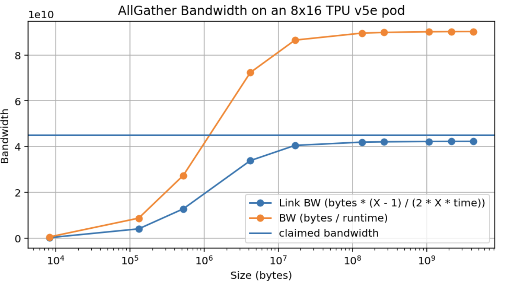
Note that we not only achieve about 95% of the peak claimed bandwidth (4.5e10) but also that we achieve this peak at about 10MB, which when 16-way sharded gives us about 625kB per device (aside: this is much better than GPUs).
注意我们不仅达到了标称峰值带宽(4.5e10)的约 95%,而且在大约 10MB 时就达到了峰值;按 16 路分片,这相当于每块设备约 625kB(顺带一提:这比 GPU 好得多)。
What happens when we AllGather over multiple axes? When we gather over multiple axes, we have multiple dimensions of ICI over which to perform the gather. For instance, AllGatherXY([B, DXY]) operates over two hardware mesh axes. This increases the available bandwidth by a factor of $N_\text{axes}$.
在多个轴上做 AllGather 会怎样? 当我们在多个轴上聚合时,就有了多个 ICI 维度可供使用。例如 AllGatherXY([B, DXY]) 会在两个硬件网格轴上操作,这会让可用带宽乘以 $N_\text{axes}$。
When considering latency, we end up with the general rule:
考虑延迟之后,我们得到一般规律:
$$T_{total} = \max \left[ \frac{T_{min} \cdot \sum_{i} |X_i|}{2}, \frac{V}{W_\text{ici} \cdot N_\text{axes}} \right]$$
where $$\sum_i \lvert X_i \rvert / 2$$ is the length of the longest path in the TPU mesh.
其中 $$\sum_i \lvert X_i \rvert / 2$$ 是 TPU 网格中最长路径的长度。
Pop Quiz 2 [AllGather time]: Using the numbers from Part 2, how long does it take to perform the AllGatherY([EY, F]) → [E, F] on a TPU v5e with a 2D mesh {'X': 8, 'Y': 4}, $$E = 2048$$, $$F = 8192$$ in bfloat16? What about with $$E=256, F=256$$?
随堂小测 2 [AllGather 耗时]: 用第 2 部分里的数字,在 TPU v5e 上、2D 网格 {'X': 8, 'Y': 4}、$$E = 2048$$、$$F = 8192$$、bfloat16 的情况下,执行 AllGatherY([EY, F]) → [E, F] 要多久?那 $$E=256, F=256$$ 呢?
Click here for the answer.
点这里看答案。
Answer: Let’s start by calculating some basic quantities:
答案: 先算几个基本量:
- TPU v5e has 4.5e10 bytes/s of unidirectional ICI bandwidth for each of its 2 axes.
- In bfloat16 for (a), we have $A[E_Y, F]$ so each device holds an array of shape bf16[512, 8192] which has 512 * 8192 * 2 = 8.4MB. The total array has size 2048 * 8192 * 2 = 34MB.
- TPU v5e 的两个轴各自有 4.5e10 bytes/s 的单向 ICI 带宽。
- bfloat16 下,情况 (a) 里我们有 $A[E_Y, F]$,所以每块设备持有的数组形状是 bf16[512, 8192],即 512 * 8192 * 2 = 8.4MB。整个数组大小是 2048 * 8192 * 2 = 34MB。
For part (1), we can use the formula above. Since we’re performing the AllGather over one axis, we have $T_{\text{comms}} = \text{34e6} / \text{9e10} = \text{377us}$. To check that we’re not latency-bound, we know over an axis of size 4, we’ll have at most 3 hops, so our latency bound is something like 3us, so we’re not close. However, TPU v5e only has a wraparound connection when one axis has size 16, so here we actually can’t do a fully bidirectional AllGather. We have to do 3 hops for data from the edges to reach the other edge, so in theory we have more like $T_{\text{comms}} = 3 * \text{8.4e6} / \text{4.5e10} = 560\mu s$. Here’s an actual profile from this Colab, which shows $680 \mu s$, which is reasonable since we’re likely not getting 100% of the theoretical bandwidth! For part (2) each shard has size 64 * 256 * 2 = 32kB. 32e3 / 4.5e10 = 0.7us, so we’re latency bound. Since we have 3 hops, this will take roughly 3 * 1us = 3us. In practice, it’s closer to 8us.
第 (1) 问:可以直接用上面的公式。因为 AllGather 只在一个轴上进行,$T_{\text{comms}} = \text{34e6} / \text{9e10} = \text{377us}$。要确认我们不是延迟受限:轴大小为 4 时最多 3 跳,延迟下界大概是 3us,所以差得很远。不过 TPU v5e 只有在某个轴大小为 16 时才有回绕(wraparound)连接,所以这里其实是做不到完全双向 AllGather 的。边缘的数据要经过 3 跳才能到另一端,理论上更接近 $T_{\text{comms}} = 3 * \text{8.4e6} / \text{4.5e10} = 560\mu s$。这里是一次真实 profile 的结果,显示 $680 \mu s$,这很合理,因为我们大概率拿不到 100% 的理论带宽!第 (2) 问:每个分片大小是 64 * 256 * 2 = 32kB. 32e3 / 4.5e10 = 0.7us,所以是延迟受限的。因为要 3 跳,大概要 3 * 1us = 3us。实践中更接近 8us。
Note: when we have a 2D mesh like {'X': 16, 'Y': 4}, it is not necessary for each axis to correspond to a specific hardware axis. This means for instance the above could describe a 4x4x4 TPU v5p cube with 2 axes on the $X$ axis. This will come into play later when we describe data parallelism over multiple axes.
注意: 像 {'X': 16, 'Y': 4} 这样的 2D 网格,并不要求每个轴对应某个特定的硬件轴。也就是说,上面的例子既可以描述一个 4x4x4 的 TPU v5p cube,其中 $X$ 轴上叠了两个轴。等后面讲到跨多个轴的数据并行时,这一点会派上用场。
Case 3: both multiplicands have sharded contracting dimensions
情况 3:两个乘数都沿收缩维度分片
The third fundamental case is when both multiplicands are sharded on their contracting dimensions, along the same mesh axis:
第三种基本情况是两个乘数都沿收缩维度分片、且沿同一个网格轴:
$$\textbf{A}[I, J_X] \cdot \textbf{B}[J_X, K] \rightarrow C[I, K]$$
In this case the local sharded block matrix multiplies are at least possible to perform, since they will share the same sets of contracting indices. But each product will only represent a partial sum of the full desired product, and each device along the X dimension will be left with different partial sums of this final desired product. This is so common that we extend our notation to explicitly mark this condition:
在这种情况下,本地的分块矩阵乘法至少是可以做的,因为它们共享同一组收缩下标。但每个乘积只代表最终结果的一个部分和,X 维度上的每块设备拿到的是不同的部分和。这种情况太常见了,所以我们扩展记号,显式标出这个状态:
$$\textbf{A}[I, J_X] \cdot_\text{LOCAL} \textbf{B}[J_X, K] \rightarrow C[I, K] \{\ U_X \}$$
The notation { UX } reads “unreduced along X mesh axis” and refers to this status of the operation being “incomplete” in a sense, in that it will only be finished pending a final sum. The $\cdot_\text{LOCAL}$ syntax means we perform the local sum but leave the result unreduced.
记号 { UX } 读作「沿 X 网格轴未归约(unreduced)」,指的是这个运算在某种意义上是「未完成」的——要等最后一次求和才算结束。$\cdot_\text{LOCAL}$ 这个写法表示我们做了本地求和,但结果尚未归约。
This can be seen as the following result about matrix multiplications and outer products:
这可以看作关于矩阵乘法和外积的下面这个结论:
$$A \cdot B = \sum_{i=1}^{P} \underbrace{A_{:,i} \otimes B_{i,:}}_{\in \mathbb{R}^{n \times m}}$$
where ⊗ is the outer product. Thus, if TPU i on axis X has the ith column of A, and the ith row of B, we can do a local matrix multiplication to obtain $$A_{:,i} \otimes B_{i,:} \in \mathbb{R}_{n\times m}$$. This matrix has, in each entry, the ith term of the sum that A • B has at that entry. We still need to perform that sum over P, which we sharded over mesh axis X, to obtain the full A • B. This works the same way if we write A and B by blocks (i.e. shards), and then sum over each resulting shard of the result.
其中 ⊗ 是外积。于是,如果 X 轴上的第 i 块 TPU 持有 A 的第 i 列和 B 的第 i 行,我们就可以做一次本地矩阵乘法得到 $$A_{:,i} \otimes B_{i,:} \in \mathbb{R}_{n\times m}$$。这个矩阵的每个元素,正是 A • B 对应元素求和中第 i 项。我们还需要对 P 求和(它被分片到网格轴 X 上),才能得到完整的 A • B。如果我们按块(即分片)写 A 和 B,再对结果的每个分片求和,道理是一样的。
We can perform this summation using a full AllReduce across the X axis to remedy this:
我们可以用一次跨 X 轴的完整 AllReduce 来完成这个求和:
$$\begin{align*} A[I, J_X] \cdot_\text{LOCAL} B[J_X, K] \rightarrow &\ C[I, K] \{ U_X \} \\ \textbf{AllReduce}_X C[I, K] \{ U_X \} \rightarrow &\ C[I, K] \end{align*}$$
AllReduce removes partial sums, resulting in each device along the axis having the same fully-summed value. AllReduce is the second of several key communications we’ll discuss in this section, the first being the AllGather, and the others being ReduceScatter and AllToAll. An AllReduce takes an array with an unreduced (partially summed) axis and performs the sum by passing those shards around the unreduced axis and accumulating the result. The signature is
AllReduce 会消除部分和,使该轴上的每块设备都得到相同的、完全归约后的值。AllReduce 是本节要讨论的第二个关键通信,第一个是 AllGather,其余还有 ReduceScatter 和 AllToAll。AllReduce 接收一个带有未归约(部分求和)轴的数组,通过把这个轴上的分片互相传递并累加,来完成求和。它的签名是
$$\textbf{AllReduce}_Y A[I_X, J] \{U_Y\} \rightarrow A[I_X, J]$$
This means it simply removes the $\\{U_Y\\}$ suffix but otherwise leaves the result unchanged.
也就是说,它只是去掉 $\\{U_Y\\}$ 后缀,其余部分保持不变。
How expensive is an AllReduce? One mental model for how an AllReduce is performed is that every device sends its shard to its neighbors, and sums up all the shards that it receives. Clearly, this is more expensive than an AllGather because each “shard” has the same shape as the full array. Generally, an AllReduce is twice as expensive as an AllGather. One way to see this is to note that an AllReduce can be expressed as a composition of two other primitives: a ReduceScatter and an AllGather. Like an AllReduce, a ReduceScatter resolves partial sums on an array but results in an output ‘scattered’ or partitioned along a given dimension. AllGather collects all those pieces and ‘unpartitions/unshards/replicates’ the logical axis along that physical axis.
AllReduce 有多贵? 一个理解 AllReduce 的心智模型是:每块设备把自己的分片发给邻居,并把收到的所有分片加起来。显然,它比 AllGather 更贵,因为这里的每个「分片」都和完整数组一样大。一般来说,AllReduce 的代价是 AllGather 的两倍。 一种理解方式是:AllReduce 可以表示成另外两个原语的组合:一次 ReduceScatter 加一次 AllGather。和 AllReduce 一样,ReduceScatter 会解决数组上的部分和,但输出是沿某个给定维度「散开」(划分)的。AllGather 则把这些碎片收集起来,把该逻辑轴在对应物理轴上「反划分 / 去分片 / 复制」。
$$\begin{align*} \textbf{ReduceScatter}_{Y,J} : A[I_X,J] \{U_Y\} \rightarrow &\ A[I_X, J_Y] \\ \textbf{AllGather}_Y : A[I_X, J_Y] \rightarrow &\ A[I_X, J] \end{align*}$$
What about a ReduceScatter? Just as the AllGather reassembles a sharded array (removing a subscript), a ReduceScatter sums an unreduced/partially summed array and then scatters (shards) a different logical axis along the same mesh axis. $X[F]\\{U_Y\\} \to X[F_Y]$. The animation shows how this is done: note that it’s very similar to an AllGather but instead of retaining each shard, we sum them together. Thus, its latency is roughly the same, excluding the time taken to perform the reduction.
那 ReduceScatter 呢? 就像 AllGather 会重新拼装分片数组(去掉一个下标),ReduceScatter 会对一个未归约/部分求和的数组求和,然后把另一个逻辑轴散开(分片)到同一个网格轴上:$X[F]\\{U_Y\\} \to X[F_Y]$。动画展示了它是怎么做的:注意它和 AllGather 非常像,只是不保留每个分片,而是把它们加起来。因此它的延迟大致相同,只是多出做归约本身的时间。
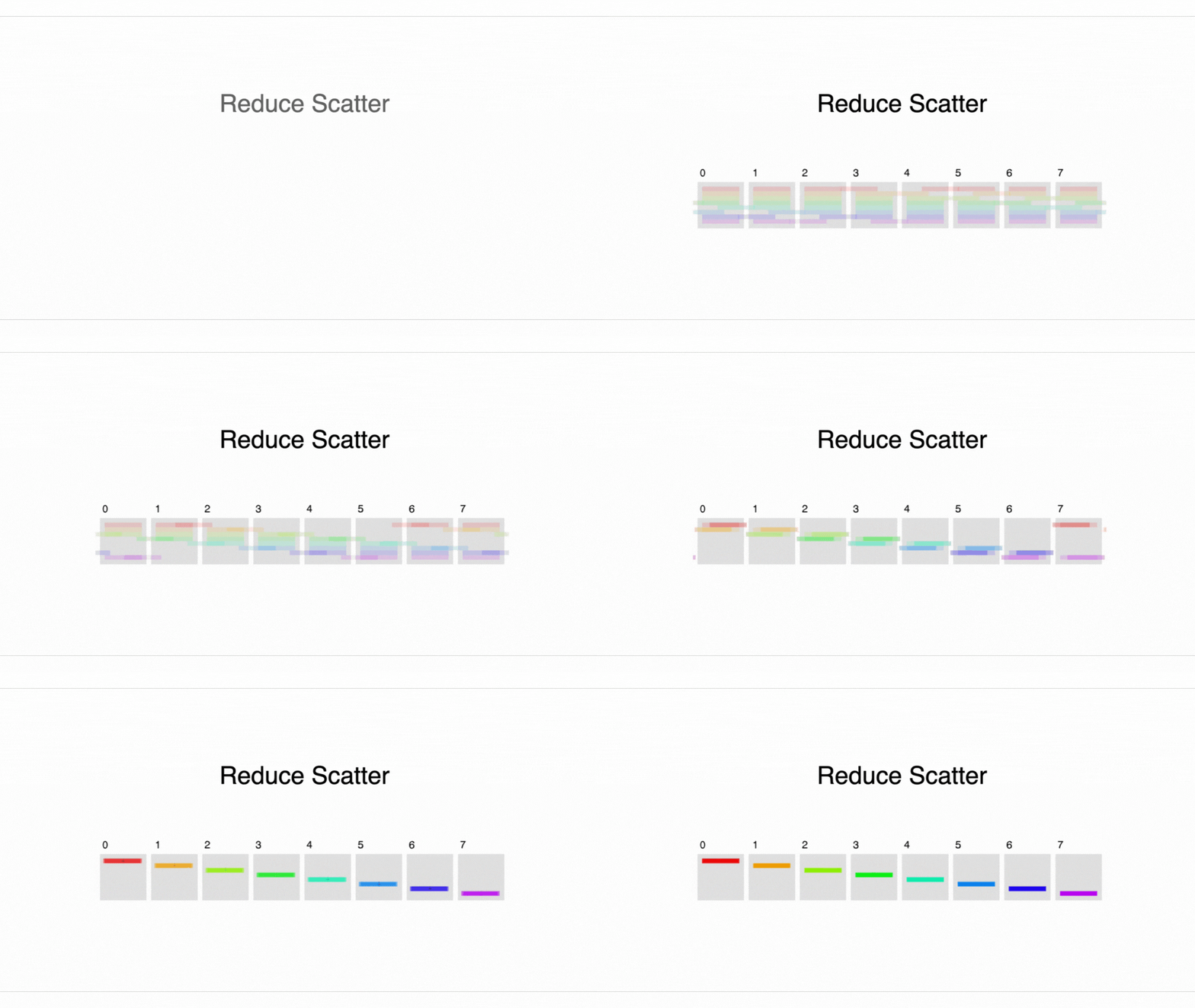
The communication time for each hop is simply the per-shard bytes $V / Y$ divided by the bandwidth $W_\text{ici}$, as it was for an AllGather, so we have
对每一跳来说,通信时间就是每分片字节数 $V / Y$ 除以带宽 $W_\text{ici}$,和 AllGather 一样,于是
$$T_{\text{comms per AllGather or ReduceScatter}} = \frac{V}{W_\text{ici}}$$
$$T_{\text{comms per AllReduce}} = 2 \cdot \frac{V}{W_\text{ici}}$$
where $$W_\text{ici}$$ is the bidirectional bandwidth, so long as we have a full ring to reduce over.
其中 $$W_\text{ici}$$ 是双向带宽,前提是我们有一个完整的环可供归约。
Case 4: both multiplicands have a non-contracting dimension sharded along the same axis
情况 4:两个乘数都有一个非收缩维度沿同一个轴分片
Each mesh dimension can appear at most once when sharding a tensor. Performing the above rules can sometimes lead to a situation where this rule is violated, such as:
在给张量分片时,每个网格维度最多只能出现一次。套用上面的规则有时会得到违反这一点的情形,例如:
$$A[I_X, J] \cdot B[J, K_X] \rightarrow C[I_X, K_X]$$
This is invalid because a given shard, say i, along dimension X, would have the **(i, i)**th shard of C, that is, a diagonal entry. There is not enough information among all shards, then, to recover anything but the diagonal entries of the result, so we cannot allow this sharding.
这是非法的:X 维度上的某个分片(比如第 i 个)只会拿到 C 的第 (i, i) 个分片,也就是对角线上的元素。所有分片合起来也不足以恢复出除对角线以外的任何信息,所以这种分片不能允许。
The way to resolve this is to AllGather some of the dimensions. Here we have two choices:
解决办法是 AllGather 掉其中一些维度。这里我们有两个选择:
$$\begin{align*} \textbf{AllGather}_X A[I_X, J] \rightarrow &\ A[I, J] \\ A[I, J] \cdot B[J, K_X] \rightarrow &\ C[I, K_X] \end{align*}$$
or
或者
$$\begin{align*} \textbf{AllGather}_X B[J, K_X] \rightarrow &\ B[J, K] \\ A[I_X, J] \cdot B[J, K] \rightarrow &\ C[I_X, K] \end{align*}$$
In either case, the result will only mention X once in its shape. Which one we pick will be based on what sharding the following operations need.
无论哪种,结果的形状里都只会出现一次 X。具体选哪个,取决于后续运算需要什么样的分片。
A Deeper Dive into TPU Communication Primitives
深入 TPU 通信原语
The previous 4 cases have introduced several “core communication primitives” used to perform sharded matrix multiplications:
前面 4 种情况引入了几个用来完成分片矩阵乘法的「核心通信原语」:
- AllGather: removes a subscript from a sharding, gathering the shards.
- ReduceScatter: removes an “un-reduced” suffix from an array by summing shards over that axis, leaving the array sharded over a second axis.
- AllReduce: removes an “un-reduced” suffix, leaving the array unsharded along that axis.
- AllGather: 去掉分片里的一个下标,把分片收集起来。
- ReduceScatter: 把数组里「未归约」的后缀去掉:在该轴上把分片求和,同时把数组分片到另一个轴上。
- AllReduce: 去掉「未归约」后缀,让数组在该轴上不再分片。
There’s one more core communication primitive to mention that arises in the case of Mixture of Experts (MoE) models and other computations: the AllToAll.
还有一些核心通信原语出现在混合专家(MoE)模型和其他计算中:AllToAll。
Our final communication primitive: the AllToAll
最后一个通信原语:AllToAll
A final fundamental collective which does not occur naturally when considering sharded matrix multiplies, but which comes up constantly in practice, is the AllToAll collective, or more precisely the special case of a sharded transposition or resharding operation. e.g.
最后一个基础集合通信,在考虑分片矩阵乘法时不会自然出现,但在实践中经常遇到,就是 AllToAll——更准确地说,是分片转置或者说重新分片操作的特例,例如
$$\textbf{AllToAll}_{X, J} A[I_X, J] \rightarrow A[I, J_X]$$
AllToAlls are typically required to rearrange sharded layouts between different regions of a sharded computation that don’t have compatible layout schemes. They arise naturally when considering sharded mixture-of-experts models. You can think of an AllToAll as moving a subscript from one axis to another. Because an all to all doesn’t need to replicate all of the data of each shard across the ring, it’s actually cheaper than an AllGather (by a factor of ¼) (For even-sized bidirectional rings, each device will send $(N/2 + (N/2-1) + … + 1)$ chunks right and $((N/2-1) + … + 1)$ chunks left $= 0.5 \cdot (N / 2) \cdot (N/2 + 1) + 0.5 \cdot (N / 2) \cdot (N/2 - 1) = N^2/4$. The size of each chunk (aka shard of a shard) is $\text{bytes} / N^2$ so the per-device cost is $(\text{bytes} / N^2) \cdot N^2 / 4 = \text{bytes} / 4$. This result scales across all devices as the total bandwidth scales with device number.).
当分片计算中不同区域的分片布局互不兼容、需要重排时,通常就得用 AllToAll。在分片混合专家模型里它自然会冒出来。你可以把 AllToAll 理解为把一个下标从一个轴搬到另一个轴。 因为 AllToAll 不需要把每个分片的数据复制到环上的所有设备,它实际上比 AllGather 更便宜(便宜到 ¼)。(对偶数大小的双向环,每块设备向右发 $(N/2 + (N/2-1) + … + 1)$ 个块、向左发 $((N/2-1) + … + 1)$ 个块 $= 0.5 \cdot (N / 2) \cdot (N/2 + 1) + 0.5 \cdot (N / 2) \cdot (N/2 - 1) = N^2/4$。每个块(也就是「分片的分片」)大小是 $\text{bytes} / N^2$,所以每块设备的代价是 $(\text{bytes} / N^2) \cdot N^2 / 4 = \text{bytes} / 4$。这个结论对所有设备都成立,因为总带宽随设备数线性增长。)

If we generalize to an ND AllToAll, the overall cost for an array of $V$ total bytes (summed across all devices) on an AxBxC mesh is
如果推广到 ND AllToAll,一个总大小 $V$ 字节(所有设备加起来)的数组在 AxBxC 网格上的总代价是
$$T_\text{comms per AllToAll} = \frac{V \cdot \max(A, B, C, ...)}{4 \cdot N \cdot W_\text{ici}}$$
where as usual $W_\text{ici}$ is the bidirectional ICI bandwidth and $N = A \cdot B \cdot C \cdot \ldots$ is the total number of devices. Equivalently, in terms of the per-device bytes $V / N$, the cost is $(V / N) \cdot \max(A, B, C, ...) / (4 \cdot W_\text{ici})$. For a 1D mesh, this reduces to $V / (4 \cdot W_\text{ici})$, which is 1 / 4 the cost of an AllGather. In 2D, the cost actually scales down with the size of the smallest axis.
其中照例 $W_\text{ici}$ 是双向 ICI 带宽,$N = A \cdot B \cdot C \cdot \ldots$ 是设备总数。等价地,用每设备字节数 $V / N$ 表示,代价是 $(V / N) \cdot \max(A, B, C, ...) / (4 \cdot W_\text{ici})$。在一维网格下它退化为 $V / (4 \cdot W_\text{ici})$,正好是 AllGather 代价的 1/4;在 2D 下,代价实际上会随最小轴的大小下降。
Aside: If you want a hand-wavy derivation of this fact, start with a 1D torus $\mathbb{Z} / N\mathbb{Z}$. If we pick a source and target node at random, they are on average N / 4 hops from each other, giving us a cost of $(V \cdot N) / (4 * N)$. Now if we consider an ND torus, each axis is basically independent. Each node has $1 / N$ bytes and on average has to hop its data $\max(A, B, C, …) / 4$ hops. You can also derive this from bisection bandwidth: in an AllToAll, each half of the mesh sends half its data ($V / 4$ bytes) to the other half. The narrowest bisection cuts perpendicular to the longest axis, crossing $2 \cdot N / \max(A, B, …)$ links (two cut planes, counting wraparound), for a one-directional bandwidth of $N \cdot W_\text{ici} / \max(A, B, …)$. Dividing gives the formula above.
顺带一提:如果你想看一个粗略的推导,可以从一维环面 $\mathbb{Z} / N\mathbb{Z}$ 出发。随机取一个源节点和目标节点,它们平均相距 N / 4 跳,代价就是 $(V \cdot N) / (4 * N)$。再考虑 ND 环面:每个轴基本独立,每个节点持有 $1 / N$ 的字节,平均要跳 $\max(A, B, C, …) / 4$ 跳。你也可以从二分带宽(bisection bandwidth)推出来:在一次 AllToAll 中,网格的每一半都要把一半数据($V / 4$ 字节)发给另一半。最窄的二分切割垂直于最长的轴,穿过 $2 \cdot N / \max(A, B, …)$ 条链路(两个切割面,含回绕),单向带宽为 $N \cdot W_\text{ici} / \max(A, B, …)$。两者相除就得到上面的公式。
More about the ReduceScatter
更多关于 ReduceScatter 的事
ReduceScatter is a more fundamental operation than it first appears, as it is actually the derivative of an AllGather, and vice versa. i.e. if in the forward pass we have:
ReduceScatter 比它初看起来更底层:它实际上是 AllGather 的导数,反之亦然。也就是说,如果前向传播是
$$\textbf{AllGather}_X A[I_X] \rightarrow A[I]$$
Then we ReduceScatter the reverse-mode derivatives A’ (which will in general be different on each shard) to derive the sharded A’:
那么我们就对反向传播的导数 A’(它在不同分片上一般不同)做 ReduceScatter,得到分片的 A’:
$$\textbf{ReduceScatter}_X A'[I] \{ U_X \} \rightarrow A'[I_X]$$
Likewise, $$\text{ReduceScatter}_X(A[I] \{U_X\}) \to A[I_X]$$ in the forward pass implies $$\text{AllGather}_{X}(A'[I_X]) \to A'[I]$$ in the backwards pass.
同样地,前向里的 $$\text{ReduceScatter}_X(A[I] \{U_X\}) \to A[I_X]$$ 对应反向里的 $$\text{AllGather}_{X}(A'[I_X]) \to A'[I]$$。
For details on how AllGather and ReduceScatter are derivatives of each other, click here.
关于 AllGather 与 ReduceScatter 互为导数的细节,点这里。
This stems from the fact that broadcasts and reductions are transposes of each other as linear operators, and AllGather and ReduceScatter are outer products (also known as Kronecker products) of broadcast and reduce, respectively. Concretely, if we have a vector $x \in \mathbb{R}^n$, any number of devices $p \in \mathbb{N}$, and we let $u = (1, \ldots, 1) \in \mathbb{R}^p$, we can define broadcast and reduce in the following way, which should match your intuitive understanding of them:
这源于一个事实:作为线性算子,广播(broadcast)和归约(reduce)互为转置,而 AllGather 和 ReduceScatter 分别是广播与归约的外积(也叫 Kronecker 积)。具体来说,设有向量 $x \in \mathbb{R}^n$、任意设备数 $p \in \mathbb{N}$,并令 $u = (1, \ldots, 1) \in \mathbb{R}^p$,我们可以这样定义广播与归约,它应该和你直觉中的理解一致:
$$ \begin{align*} \text{broadcast} &: \mathbb{R}^n \rightarrow \mathbb{R}^{p n} \\ \text{broadcast} &= u \otimes \mathbf{I}_n \\ \text{reduce} &: \mathbb{R}^{p n} \rightarrow \mathbb{R}^n \\ \text{reduce} &= u^T \otimes \mathbf{I}_n \end{align*} $$
Let’s see how this looks in an example, where $n = 1$, $p = 2$. If $x = (7)$, we have $$\text{broadcast}(x) = \left(\begin{pmatrix} 1 \\ 1 \end{pmatrix} \otimes \begin{pmatrix} 1 \end{pmatrix}\right) x = \begin{pmatrix} 1 \\ 1 \end{pmatrix} x = \begin{pmatrix} 7\\ 7 \end{pmatrix} \in \mathbb{R}^{p n}$$. This matches what we’d expect, broadcasting a vector in $\mathbb{R}^n$ to $\mathbb{R}^{pn}$. Now letting $y = (8, 9)$, we have $$\text{reduce}(y) = \left(\begin{pmatrix} 1 & 1 \end{pmatrix} \otimes \begin{pmatrix} 1\end{pmatrix}\right) y = \begin{pmatrix} 1 & 1 \end{pmatrix} \begin{pmatrix} 8 \\ 9 \end{pmatrix} = \begin{pmatrix} 17 \end{pmatrix}$$. This again matches what we’d expect, reducing a vector in $\mathbb{R}^{p n}$ to a vector in $\mathbb{R}^{n}$. Since $(A \otimes B)^T = A^T \otimes B^T$ for any two matrices $A$ and $B$, we see that $\text{reduce} = \text{broadcast}^T$. We recover AllGather and ReduceScatter as the following outer products:
看个例子:$n = 1$,$p = 2$。如果 $x = (7)$,那么 $$\text{broadcast}(x) = \left(\begin{pmatrix} 1 \\ 1 \end{pmatrix} \otimes \begin{pmatrix} 1 \end{pmatrix}\right) x = \begin{pmatrix} 1 \\ 1 \end{pmatrix} x = \begin{pmatrix} 7\\ 7 \end{pmatrix} \in \mathbb{R}^{p n}$$。这符合预期:把一个 $\mathbb{R}^n$ 的向量广播成 $\mathbb{R}^{pn}$。再令 $y = (8, 9)$,有 $$\text{reduce}(y) = \left(\begin{pmatrix} 1 & 1 \end{pmatrix} \otimes \begin{pmatrix} 1\end{pmatrix}\right) y = \begin{pmatrix} 1 & 1 \end{pmatrix} \begin{pmatrix} 8 \\ 9 \end{pmatrix} = \begin{pmatrix} 17 \end{pmatrix}$$。同样符合预期:把一个 $\mathbb{R}^{p n}$ 的向量归约成 $\mathbb{R}^{n}$ 的向量。由于对任意两个矩阵 $A$ 和 $B$ 都有 $(A \otimes B)^T = A^T \otimes B^T$,我们看到 $\text{reduce} = \text{broadcast}^T$。于是 AllGather 和 ReduceScatter 可以写成如下的外积:
$$ \begin{align*} \text{AllGather} &: \mathbb{R}^{p n} \rightarrow \mathbb{R}^{p^2 n} \\ \text{AllGather} &= \text{broadcast} \otimes \mathbf{I}_p \\ \text{ReduceScatter} &= \mathbb{R}^{p^2 n} \rightarrow \mathbb{R}^{p n} \\ \text{ReduceScatter} &= \text{reduce} \otimes \mathbf{I}_p \end{align*} $$
Here we think of $\mathbb{R}^{p^2 n}$ as $\mathbb{R}^{p \times p n}$, so one $\mathbb{R}^{p n}$ vector for each of our $p$ devices. We suggest playing around with small examples, say $n = 2$, $p = 3$, to see what these operators look like as matrices. Using the same transposition property, we once more obtain $\text{AllGather}^T = \text{ReduceScatter}$, and of course $\text{ReduceScatter}^T = \text{AllGather}$. This transposition will arise during backpropagation, since if we have $y = Ax$ for some linear operator $A$, such as AllGather or ReduceScatter, then during backpropagation we will have the derivative of the loss with respect to $y$, $\frac{\partial L}{\partial y}$, and we obtain $\frac{\partial L}{\partial x}$ as $\frac{\partial L}{\partial x} = A^T \frac{\partial L}{\partial y}$. This shows how the derivative of AllGather will be ReduceScatter, and vice versa.
这里我们把 $\mathbb{R}^{p^2 n}$ 看成 $\mathbb{R}^{p \times p n}$,也就是 $p$ 块设备各对应一个 $\mathbb{R}^{p n}$ 向量。建议你拿小例子(比如 $n = 2$、$p = 3$)动手玩一玩,看看这些算子写成矩阵长什么样。利用同样的转置性质,我们再次得到 $\text{AllGather}^T = \text{ReduceScatter}$,当然也有 $\text{ReduceScatter}^T = \text{AllGather}$。这个转置会在反向传播中出现:如果对某个线性算子 $A$(比如 AllGather 或 ReduceScatter)有 $y = Ax$,那么反向传播时我们已知损失对 $y$ 的导数 $\frac{\partial L}{\partial y}$,并由此得到 $\frac{\partial L}{\partial x} = A^T \frac{\partial L}{\partial y}$。这就说明了 AllGather 的导数是 ReduceScatter,反之亦然。
Turning an AllReduce into an AllGather and ReduceScatter also has the convenient property that we can defer the final AllGather until some later moment. Very commonly we’d rather not pay the cost of reassembling the full matrix product replicated across the devices. Rather we’d like to preserve a sharded state even in this case of combining two multiplicands with sharded contracting dimensions:
把 AllReduce 拆成 AllGather + ReduceScatter 还有一个方便之处:我们可以把最后的 AllGather 推迟到之后再做。很多时候我们并不想为「把完整矩阵乘积在各设备上复制一遍」付出代价,而是希望即使在这种「两个乘数都沿收缩维度分片」的情况下,也保持一份分片状态:
$$A[I, J_X] \cdot B[J_X, K] \rightarrow C[I, K_X]$$
In this case, we can also perform a ReduceScatter instead of an AllReduce, and then optionally perform the AllGather at some later time, i.e.
这种情况下,我们可以用 ReduceScatter 代替 AllReduce,之后需要时再补一次 AllGather,也就是
$$\begin{align*} A[I, J_X] \cdot_{LOCAL} B[J_X, K] \rightarrow &\ C[I, K] \{ U_X \} \\ \textbf{ReduceScatter}_{X,K} C[I, K] \{ U_X \} \rightarrow &\ C[I, K_X] \end{align*}$$
Note that ReduceScatter introduces a sharded dimension, and so has a natural freedom to shard along either the I or K named dimensions in this case. We generally need to choose which named dimension to introduce a new sharding to when using a ReduceScatter (though the choice is usually forced by the larger modeling context). This is why we use the syntax ReduceScatterX,K to specify the axis to shard.
注意 ReduceScatter 会引入一个分片维度,因此这里天然有自由选择把它分到 I 还是 K 命名维度上。使用 ReduceScatter 时,我们通常要选择引入新的分片到哪个命名维度(不过这个选择往往被更大的建模上下文所限定)。这就是我们用 ReduceScatterX,K 这种写法来指定分片轴的原因。
How to overlap matmul communication with compute
如何让矩阵乘法的通信与计算重叠
As we discussed in Part 1, we generally assume we can always overlap communication with some useful computation if the comms are fast enough. The collectives in this section generally can be overlapped with the matrix multiplication compute itself, but doing so is non-trivial. The algorithm we use is something called a collective matmul, first described in Wang et al.. Here is a simplified animation of how this overlap can be implemented:
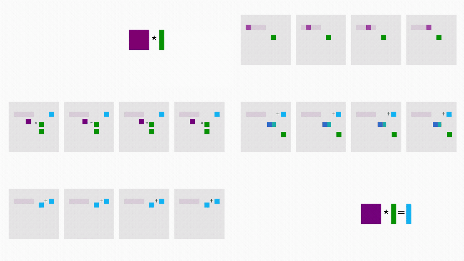
To put it simply, we can do the matmul for one chunk of the matrix while starting the ring reduction for previous chunks. In some cases we can also tile over the batch dimension or matrix input dimension. We work through a simple JAX implementation in Part 10 and the Mosaic docs also give a good example on GPU. We encourage you to implement a version of this at some point.
What Have We Learned?
我们学到了什么?
- The sharding of an array is specified by a Mesh that names the physical, hardware axes of our TPU mesh and a Sharding that assigns mesh axis names to the logical axes of the array.
- For example, A[IXY, J] describes an abstract array A with its first dimension sharded along two mesh axes X and Y. Combined with Mesh(mesh_shape=(4, 8), axis_names=(‘X’, ‘Y’)) or the abbreviated Mesh({‘X’: 4, ‘Y’: 8}), this tells us our array is sharded 32 ways along the first dimension.
- 数组的分片由一个 Mesh 和一个 Sharding 共同指定:前者命名 TPU 网格的物理硬件轴,后者把网格轴名分配给数组的逻辑轴。
- 例如 A[IXY, J] 描述一个抽象数组 A,它的第一个维度沿 X、Y 两个网格轴分片。配合 Mesh(mesh_shape=(4, 8), axis_names=(‘X’, ‘Y’)),或缩写 Mesh({‘X’: 4, ‘Y’: 8}),这告诉我们数组的第一个维度被分成 32 份。
- Arithmetic with sharded arrays works exactly like with unsharded arrays unless you perform a contraction along a sharded axis. In that case, we have to introduce some communication. We consider four cases:
- 只要不在分片轴上做收缩,分片数组的算术运算就和未分片数组完全一样。一旦在分片轴上收缩,就必须引入通信。我们考虑四种情况:
- Neither array is sharded along the contracting dimension: no communication is needed.
- One array is sharded along the contracting dimension (or the contracting dimensions are sharded along different axes): we AllGather one of the inputs before performing the operation.
- Both arrays are identically sharded along the contracting dimension: we multiply the shards locally then perform an AllReduce or ReduceScatter.
- Both arrays are sharded along the same mesh axis along a non-contracting dimension: we AllGather one of the inputs first.
- 两个数组都不沿收缩维度分片:不需要通信。
- 一个数组沿收缩维度分片(或两个收缩维度分片在不同轴上):先对其中一个输入做 AllGather,再做运算。
- 两个数组沿收缩维度同样地分片:先本地相乘分片,然后做 AllReduce 或 ReduceScatter。
- 两个数组都有一个非收缩维度沿同一个网格轴分片:先对其中一个输入做 AllGather。
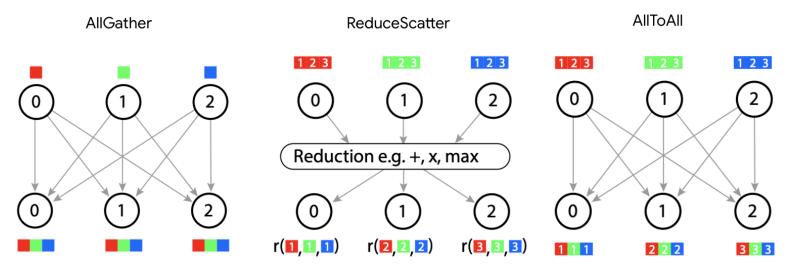
- TPUs use roughly 4 core communication primitives:
- TPU 大致有 4 个核心通信原语:
- AllGather: $[A_X, B] \to [A, B]$
- ReduceScatter: $[A, B] \\{U_X\\} \to [A_X, B]$
- AllToAll: $[A, B_X] \to [A_X, B]$
- AllReduce: $[A_X, B]\\{U_Y\\} \to [A_X, B]$ (technically not a primitive since it combines a ReduceScatter + AllGather)
- AllGather:$[A_X, B] \to [A, B]$
- ReduceScatter:$[A, B] \\{U_X\\} \to [A_X, B]$
- AllToAll:$[A, B_X] \to [A_X, B]$
- AllReduce:$[A_X, B]\\{U_Y\\} \to [A_X, B]$(严格来说不算原语,因为它由 ReduceScatter + AllGather 组合而成)
- The cost and latency of each of these operations doesn’t depend on the size of the axis (as long as they’re bandwidth bound), but only on the size of the input arrays and the bandwidth of the link. For a unidirectional AllGather/ReduceScatter:
- 这些操作的代价和延迟不取决于轴的大小(只要处在带宽受限区间),只取决于输入数组的大小和链路带宽。对单向 AllGather/ReduceScatter:
$$T_{\text{comm per AllGather or ReduceScatter}} = \frac{\text{Data volume}}{\text{bandwidth}} \cdot \frac{\text{Axis} - 1}{\text{Axis}} \longrightarrow \frac{\text{Data volume}}{\text{bandwidth (bidirectional)}}$$
- An AllReduce is composed of a ReduceScatter followed by an AllGather, and thus has 2x the above cost. An AllToAll only has to pass shards part-way around the ring and is thus ¼ the cost of an AllGather. Here’s a summary:
- 一次 AllReduce 由一次 ReduceScatter 加一次 AllGather 组成,因此代价是上面的 2 倍。AllToAll 只需要把分片沿环传递一部分,因此代价是 AllGather 的 ¼。下面是汇总:
| Operation | Description | Syntax | Runtime |
|---|---|---|---|
| AllGather | Gathers all the shards of a sharded array along an axis, removing a subscript. | $[A_X, B] \to [A, B]$ | bytes / (bidirectional ICI bandwidth * num_axes) |
| ReduceScatter | Sums a partially summed array along an axis and shards it along another axis (adding a subscript). | $[A, B] \\{U_X\\} \to [A_X, B]$ | Same as AllGather |
| AllReduce | Sums a partially summed array along an axis. Removes a { Ux }. Combines an AllGather and ReduceScatter. | $[A_X, B]\\{U_Y\\} \to [A_X, B]$ | 2 * AllGather |
| AllToAll | Gathers (replicates) an axis and shards a different dimension along the same axis. | $[A, B_X] \to [A_X, B]$ | AllGather / 4 for a bidirectional ring |
Some Problems to Work
一些练习题
Here are some instructive problems based on content in this section. We won’t include all answers at the moment but we’ll write up more answers as we can.
下面是基于本节内容的一些有启发性的题目。我们暂时不会给出所有答案,但会尽量多写一些。
Question 1 [replicated sharding]: An array is sharded $A[I_X, J, K, \ldots]$ (i.e., only sharded across $X$), with a mesh Mesh({'X': 4, 'Y': 8, 'Z': 2}). What is the ratio of the total number of bytes taken up by $A$ across all chips to the size of one copy of the array?
第 1 题 [复制分片]:一个数组分片为 $A[I_X, J, K, \ldots]$(即只沿 $X$ 分片),网格是 Mesh({'X': 4, 'Y': 8, 'Z': 2})。$A$ 在所有芯片上占用的总字节数,与数组单份拷贝的大小之比是多少?
Click here for the answer.
点这里看答案。
Our array is only sharded along X, which has size 4, so effectively each shard has size $[I / 4, J, K, \ldots] = \text{sizeof}(A) / 4$. Since our array is replicated across Y and Z, the total size is $Y \cdot Z \cdot \text{sizeof}(A)$, so the ratio of total size to single chip size is $Y \cdot Z \cdot \text{sizeof}(A) / \text{sizeof}(A) = 16$.
我们的数组只沿 X 分片,X 大小为 4,所以每个分片大小是 $[I / 4, J, K, \ldots] = \text{sizeof}(A) / 4$。由于数组在 Y 和 Z 上被复制,总大小是 $Y \cdot Z \cdot \text{sizeof}(A)$,所以总大小与单芯片大小的比值是 $Y \cdot Z \cdot \text{sizeof}(A) / \text{sizeof}(A) = 16$。
Question 2 [AllGather latency]: How long should $\text{AllGather}_X([B_X, D_Y])$ take on a TPU v4p 4x4x4 slice with mesh Mesh({'X': 4, 'Y': 4, 'Z': 4}) if $B=1024$ and $D=4096$ in bfloat16? How about $$\text{AllGather}_{XY}([B_X, D_Y])$$? How about $$\text{AllReduce}_Z([B_X, D_Y] \{U_Z \})$$?
第 2 题 [AllGather 延迟]:在 TPU v4p 4x4x4 slice、网格 Mesh({'X': 4, 'Y': 4, 'Z': 4})、$B=1024$、$D=4096$、bfloat16 的情况下,$\text{AllGather}_X([B_X, D_Y])$ 应该花多久?$$\text{AllGather}_{XY}([B_X, D_Y])$$ 呢?$$\text{AllReduce}_Z([B_X, D_Y] \{U_Z \})$$ 呢?
Click here for the answer.
点这里看答案。
We have a wraparound link on all axes because we have a full 4x4x4 cube, so we have 9e10 bidirectional bandwidth to work with.
因为是一个完整的 4x4x4 cube,所有轴都有回绕连接,所以可用带宽是 9e10(双向)。
- Because we’re just gathering over one axis and the other is sharded, we’re effectively gathering $2BD / Y$ bytes over 1 axis. If you think about just a single shard along the Y-axis, the AllGather along X looks like an unsharded AllGather with 1 / Y of the bytes. Since our ICI bandwidth for TPU v4p is 9e10 bytes/second bidirectional, this will take $2BD / (\text{9e10} \cdot Y) = 2 \cdot 1024 \cdot 4096 / (\text{9e10} \cdot 4) = 23 \mu s$.
- 因为我们只在一个轴上聚合,另一个轴保持分片,所以实际上是沿 1 个轴聚合 $2BD / Y$ 字节。如果你只盯着 Y 轴上的单个分片,沿 X 的 AllGather 看起来就像一次字节数为 1/Y 的未分片 AllGather。 TPU v4p 的 ICI 带宽是 9e10 bytes/s(双向),所以耗时 $2BD / (\text{9e10} \cdot Y) = 2 \cdot 1024 \cdot 4096 / (\text{9e10} \cdot 4) = 23 \mu s$。
- We have twice the bandwidth as before but we’re AllGathering the full array, so
T = 2BD / (2 * W) = 2*1024*4096 / (2 * 9e10) = 46us. This is far from the latency bound of 4us (1us per hop), so we’re fine.
- 带宽是之前的两倍,但我们要 AllGather 整个数组,所以
T = 2BD / (2 * W) = 2*1024*4096 / (2 * 9e10) = 46us。这离 4us 的延迟下界(每跳 1us)还差得远,所以我们没问题。
- The cost of an AllReduce is twice that of an AllGather. Each shard has size $2BD / (X * Y)$, so the cost is about $4BD / (X * Y * W)$, or roughly
4 * 1024 * 4096 / (16 * 9e10) = 11.6us.
- AllReduce 的代价是 AllGather 的两倍。每个分片大小是 $2BD / (X * Y)$,所以代价约为 $4BD / (X * Y * W)$,大致是
4 * 1024 * 4096 / (16 * 9e10) = 11.6us。
Fun fact: parts (1) and (2) aren’t actually optimal, because the array is also replicated along the unused Z axis, and we can exploit those idle links: we can first re-shard $[B_X, D_Y] \to [B_{XZ}, D_Y]$ for free (each device just drops part of its shard) and then perform $$\text{AllGather}_{XZ}$$ (or $$\text{AllGather}_{XYZ}$$), reaching the same final state while gathering over more axes. This cuts part (1) to 11.5us and part (2) to 31us — in practice you’d get this by just sharding over more axes up front, which is one reason to shard arrays as finely as possible.
有趣的事实: 第 (1)、(2) 问其实不是最优的,因为数组还在没用到的 Z 轴上复制,我们可以利用那些空闲链路:先免费地把 $[B_X, D_Y] \to [B_{XZ}, D_Y]$ 重新分片(每块设备丢掉自己分片的一部分),然后做 $$\text{AllGather}_{XZ}$$(或 $$\text{AllGather}_{XYZ}$$),在更多轴上聚合,达到同样的最终状态。这样第 (1) 问降到 11.5us,第 (2) 问降到 31us——实践中你只要一开始就分片到更多轴上就能拿到这个收益,这也是「尽量细地分片数组」的理由之一。
Question 3 [latency-bound AllGather]: Let’s say we’re performing an $\text{AllGather}_X([B_X])$ but $B$ is very small (say 128). How long should this take on a TPU v4p 4x4x4 slice with mesh Mesh({'X': 4, 'Y': 4, 'Z': 4}) in bfloat16? Hint: you’re probably latency bound.
第 3 题 [延迟受限的 AllGather]:假设我们要做 $\text{AllGather}_X([B_X])$,但 $B$ 非常小(比如 128)。在 TPU v4p 4x4x4 slice、网格 Mesh({'X': 4, 'Y': 4, 'Z': 4})、bfloat16 下应该花多久?提示:你大概率是延迟受限的。
Click here for the answer.
点这里看答案。
Our array in bfloat16 uses only 256 bytes total, and only 64 per device. Since we have an axis of size 4 on a TPU v4p, we have a wraparound link, so we can send the array in both directions. With 4.5e10 of unidirectional bandwidth, each hop would take roughly 64 / 4.5e10 ~ 0, so we’re definitely latency bound. Counting the number of hops, we can do the full gather in only 2 hops, so roughly 2us a good estimate.
我们的数组在 bfloat16 下总共只有 256 字节,每块设备只有 64 字节。由于在 TPU v4p 上轴大小为 4,有回绕连接,所以可以双向发送。单向带宽 4.5e10 时,每跳耗时大致 64 / 4.5e10 ~ 0,所以肯定是延迟受限。数一数跳数,整个聚合只要 2 跳,所以 2us 左右是个不错的估计。
Question 4 [matmul strategies]: To perform $X[B, D] \cdot_D Y[D_X, F] \to Z[B, F]$, in this section we tell you to perform $\text{AllGather}_X(Y[D_X, F])$ and multiply the fully replicated matrices (Case 2, Strategy 1). Instead, you could multiply the local shards like $X[B, D_X] \cdot_D Y[D_X, F] \to Z[B, F] \\{U_X\\}$ (Case 3, Strategy 2), and then $\text{AllReduce}_X(Z[B, F] \\{ U_X\\})$. How many FLOPs and comms does each of these perform? Which is better and why?
第 4 题 [矩阵乘法策略]:要完成 $X[B, D] \cdot_D Y[D_X, F] \to Z[B, F]$,本节告诉你先做 $\text{AllGather}_X(Y[D_X, F])$,然后用完全复制的矩阵相乘(情况 2,策略 1)。另一种做法是先按本地分片相乘,即 $X[B, D_X] \cdot_D Y[D_X, F] \to Z[B, F] \\{U_X\\}$(情况 3,策略 2),然后做 $\text{AllReduce}_X(Z[B, F] \\{ U_X\\})$。这两种做法各做了多少 FLOPs 和多少通信?哪个更好,为什么?
Click here for the answer.
点这里看答案。
Let’s start with our baseline (Strategy 1). As we’ve shown, the cost of the AllGather is $2DF / W_\text{ici}$. Once we have the fully replicated arrays, the total compute time is $2BDF / C$ (where $C$ is our accelerator FLOPs/s, since each TPU does the same FLOPs). So we have
先看基线(策略 1)。如我们所示,AllGather 的代价是 $2DF / W_\text{ici}$。一旦有了完全复制的数组,总计算时间是 $2BDF / C$($C$ 是加速器的 FLOPs/s,因为每块 TPU 做同样多的 FLOPs)。于是
$$T_\text{total (Strategy 1)} = \max\left(\frac{2BDF}{C}, \frac{2DF}{W_\text{ici}}\right)$$
By comparison, the new strategy (Strategy 2) does an AllReduce over $2BF$ bytes, which has cost $4BF / W_\text{ici}$ but does $1 / X$ fewer FLOPs (since the computation is sharded). This means we do $2\cdot B\cdot D\cdot F / X$ FLOPs and the resulting AllReduce communicates $$2 \cdot 2 \cdot B \cdot F$$ bytes in bfloat16. Thus, our total time for Strategy 2 (no AllGather, just an AllReduce later on) is roughly
相比之下,新策略(策略 2)对 $2BF$ 字节做 AllReduce,代价是 $4BF / W_\text{ici}$,但 FLOPs 少了 $1 / X$(因为计算被分片了)。也就是说我们做 $2\cdot B\cdot D\cdot F / X$ 次 FLOPs,而最终的 AllReduce 要通信 $$2 \cdot 2 \cdot B \cdot F$$ 字节(bfloat16)。因此策略 2 的总时间(不做 AllGather,只做一次 AllReduce)大致是
$$T_\text{total} = \max\left(\frac{2BDF}{X \cdot C}, \frac{4BF}{W_\text{ici}}\right)$$
The question is: which of these is bigger? Strategy (2) is compute bound when $D / (X \cdot C) > 2 / W_\text{ici}$, or when $D / 2X > C / W_\text{ici} \approx 2550 \rightarrow X < D / (2 * 2550)$. We might reasonably expect $D \approx 8k$, so this would mean roughly $X < 2$ which is unlikely – hence we’re basically always comms bound with Strategy 2. With the baseline (Strategy 1), we’re comms bound when $$B < C / W_\text{ici} = 2550$$ which is often but not always true.
问题是:这两个哪个更大? 策略 2 在 $D / (X \cdot C) > 2 / W_\text{ici}$,也就是 $D / 2X > C / W_\text{ici} \approx 2550 \rightarrow X < D / (2 * 2550)$ 时是计算受限的。我们可以合理地假设 $D \approx 8k$,那大致要求 $X < 2$,不太可能——所以策略 2 基本上总是通信受限。对基线(策略 1),当 $$B < C / W_\text{ici} = 2550$$ 时是通信受限,这经常成立但并非总是。
So if $B < 2550$, we’re comms-bound in both cases and we have
所以如果 $B < 2550$,两种策略都是通信受限,于是
$$T_\text{comms for Strategy 2} < T_\text{comms for Strategy 1} \Leftrightarrow \frac{4BF}{W_\text{ici}} < \frac{2DF}{W_\text{ici}}$$
which is true when $D > 2B$ where $2B < 5100$. This is often true, so Strategy 2 can sometimes be better if our batch is small. When our batch is large ($B > 2550$), we have
当 $D > 2B$(且 $2B < 5100$)时成立。这通常成立,所以 batch 较小时策略 2 有时更好。当 batch 很大($B > 2550$)时,我们有
$$T_\text{comms for Strategy 2} < T_\text{math for Strategy 1} \Leftrightarrow \frac{4BF}{W_\text{ici}} < \frac{2BDF}{C}$$
This is true when $2 / W_\text{ici} < D / C$, or when $D > 2 * 2550 = 5100$, which is usually true for large models. So this alternative strategy is typically better for large models, unless $D$ is small.
当 $2 / W_\text{ici} < D / C$,即 $D > 2 * 2550 = 5100$ 时成立,对大模型来说通常成立。所以对 D 不太小的大模型,这个替代策略通常更好。
Why don’t we always do this? Well, in practice we may do this sometimes, but it’s typically rare to have the contracting dimension of one of the inputs to a matmul sharded along an axis that the other input isn’t sharded over. For instance, if we’re doing FSDP (explained in Section 5), we’ll shard our parameters over the data dimension but our activations will also be sharded along data. So in this sense this doesn’t show up much.
那为什么不总是这么做? 实践中我们有时确实会这么做,但「某个矩阵乘法的收缩维度被分片、而另一个输入没在该轴上分片」这种情况本身很罕见。比如做 FSDP(第 5 节会讲)时,我们会把参数沿数据维度分片,而激活也沿数据分片。所以从这个意义上说,这种情形并不多见。
Question 5 [minimum latency]: Let’s say I want to do a matmul $A[I, J] \cdot_J B[J, K] \to C[I, K]$ on a TPU v4p 4x4x4 with the lowest possible latency. Assume the inputs can be sharded arbitrarily but the result should be fully replicated. How should my inputs be sharded? What is the total FLOPs and comms time?
第 5 题 [最小延迟]:假设我想在 TPU v4p 4x4x4 上以尽可能低的延迟完成矩阵乘法 $A[I, J] \cdot_J B[J, K] \to C[I, K]$。假设输入可以任意分片,但结果必须完全复制。输入该怎么分片?总的 FLOPs 和通信时间各是多少?
Click here for the (partial) answer.
点这里看(部分)答案。
We won’t provide a full answer here, but we’ll start by describing the four most likely options:
这里我们不给完整答案,先列出四种最可能的方案:
- $A[I_{XYZ}, J] \cdot B[J, K]$ + AG at the end
- $A[I, J] \cdot B[J, K_{XYZ}]$ + AG at the end
- $A[I, J_{XYZ}] \cdot B[J_{XYZ}, K]$ + AR at the end
- $A[I, J] \cdot B[J, K]$ (fully replicated)
- $A[I_{XYZ}, J] \cdot B[J, K]$ + 最后做 AG
- $A[I, J] \cdot B[J, K_{XYZ}]$ + 最后做 AG
- $A[I, J_{XYZ}] \cdot B[J_{XYZ}, K]$ + 最后做 AR
- $A[I, J] \cdot B[J, K]$(完全复制)
We could also consider sharding different axes along different mesh axes, but that isn’t likely to change the final cost. For all but (4), the total FLOPs per TPU is the same, but comms are different for each. We then simply need to calculate the comms cost for each and see which is lowest. The TLDR is that (1) and (2) are equally good.
我们也可以考虑把不同轴分到不同网格轴上,但这不太会改变最终代价。除 (4) 以外,每块 TPU 的总 FLOPs 相同,但通信各不相同。于是我们只需算出各自的通信代价,取最小的那个。结论是:(1) 和 (2) 一样好。
Question 6: Let’s say we want to perform $A[I_X, J_Y] \cdot_J B[J_Y, K] \to C[I_X, K]$ on TPU v5e 4x4. What communication do we perform? How much time is spent on communication vs. computation?
第 6 题: 假设要在 TPU v5e 4x4 上完成 $A[I_X, J_Y] \cdot_J B[J_Y, K] \to C[I_X, K]$。我们要做哪些通信?通信和计算各花多少时间?
- What about $A[I_X, J] \cdot_J B[J_X, K_Y] \to C[I_X, K_Y]$? This is the most standard setting for training where we combine data, tensor, and ZeRO sharding.
- What about $A[I_X, J] \cdot_J B[J, K_Y] \to C[I_X, K_Y]$? This is standard for inference, where we do pure tensor parallelism (+data).
- 那 $A[I_X, J] \cdot_J B[J_X, K_Y] \to C[I_X, K_Y]$ 呢?这是训练中最标准的配置,数据并行、张量并行和 ZeRO 分片在这里组合起来。
- 那 $A[I_X, J] \cdot_J B[J, K_Y] \to C[I_X, K_Y]$ 呢?这是推理的标准做法,纯张量并行(加数据并行)。
Question 7: A typical Transformer block has two matrices $W_\text{in}[D, F]$ and $W_\text{out}[F, D]$ where $F \gg D$. Say we have a batch size B. Then the full block is $In[B, D] \cdot W_\text{in}[D, F] \cdot W_\text{out}[F, D]$. Let’s pick $D=8192$, $F=32768$, and $B=128$ and assume everything is in bfloat16. Assume we’re running on a TPU v5e 2x2 slice but let’s pretend each TPU only has 300MB of free memory. How should In, $W_\text{in}$, $W_\text{out}$, and Out be sharded to stay below the memory limit while minimizing overall time? How much time is spent on comms and FLOPs? Hint: the final output doesn’t need to be fully replicated, but it should be sharded the same as the input so the “layer” can be repeated.
第 7 题: 一个典型的 Transformer block 有两个矩阵 $W_\text{in}[D, F]$ 和 $W_\text{out}[F, D]$,其中 $F \gg D$。设 batch size 为 B,那么整个 block 是 $In[B, D] \cdot W_\text{in}[D, F] \cdot W_\text{out}[F, D]$。取 $D=8192$、$F=32768$、$B=128$,一切按 bfloat16 算。假设跑在 TPU v5e 2x2 slice 上,但假装每块 TPU 只有 300MB 空闲内存。In、$W_\text{in}$、$W_\text{out}$、Out 该怎么分片,才能既不超过内存上限、又让总时间最短?通信和 FLOPs 各花多少时间?提示:最终输出不需要完全复制,但要和输入分片方式一致,这样这个「层」才能重复堆叠。
Click here for the (partial) answer.
点这里看(部分)答案。
First let’s think about memory. Each of our two big matrices uses 2 * 8192 * 32768 = 536MB. Our activations In have size 2 * 128 * 8192 = 2MB (small enough not to worry about). Since we only have 300MB of spare memory in each device, we clearly need to shard our matmuls.
先想想内存。两个大矩阵各占 2 * 8192 * 32768 = 536MB。激活 In 大小是 2 * 128 * 8192 = 2MB(足够小,不用担心)。既然每块设备只有 300MB 空闲内存,显然需要把矩阵乘法分片。
- $In[B_X, D] * W_\text{in}[D_{XY}, F] * W_\text{out}[F, D_{XY}] \rightarrow Out[B_X, D]$ (this is often called FSDP)
- $In[B, D_{XY}] * W_\text{in}[D, F_{XY}] * W_\text{out}[F_{XY}, D] \rightarrow Out[B, D_{XY}]$ (this is called tensor parallelism)
- $In[B_X, D] * W_\text{in}[D_{XY}, F] * W_\text{out}[F, D_{XY}] \rightarrow Out[B_X, D]$(这通常叫 FSDP)
- $In[B, D_{XY}] * W_\text{in}[D, F_{XY}] * W_\text{out}[F_{XY}, D] \rightarrow Out[B, D_{XY}]$(这叫做张量并行)
The first is pretty bad because we need to AllGather our big weights or our activations first. The second requires an AllGather at the beginning and a ReduceScatter at the end (which is cheaper than an AllReduce). I’ll leave it as an exercise to do the rest of the math.
第一种相当糟糕,因为需要先把大权重或激活 AllGather 起来。第二种需要在开头做一次 AllGather、结尾做一次 ReduceScatter(比 AllReduce 便宜)。剩下的数学就留作练习吧。
Question 8 [challenge]: Using the short code snippet above as a template, allocate a sharded array and benchmark each of the 4 main communication primitives (AllGather, AllReduce, ReduceScatter, and AllToAll) using pmap or shard_map. You will want to use jax.lax.all_gather, jax.lax.psum, jax.lax.psum_scatter, and jax.lax.all_to_all. Do you understand the semantics of these functions? How long do they take?
第 8 题 [挑战]:以上面的小代码片段为模板,分配一个分片数组,用 pmap 或 shard_map 对 4 个主要通信原语(AllGather、AllReduce、ReduceScatter、AllToAll)逐个 benchmark。你会用到 jax.lax.all_gather、jax.lax.psum、jax.lax.psum_scatter 和 jax.lax.all_to_all。你理解这些函数的语义吗?它们各要多久?
Question 9 [another strategy for sharded matmuls?]: Above we claimed that when only one input to a matmul is sharded along its contracting dimension, we should AllGather the sharded matrix and perform the resulting contraction locally. Another strategy you might think of is to perform the sharded matmul and then AllReduce the result (as if both inputs were sharded along the contracting dimension), i.e. $A[I, J_X] *_J B[J, K] \to C[I, K]$ by way of
第 9 题 [分片矩阵乘法的另一种策略?]:前面我们说过,当矩阵乘法只有一个输入沿收缩维度分片时,我们应该把分片的矩阵 AllGather 起来,再做本地收缩。你可能还会想到另一种策略:先做分片的矩阵乘法,然后对结果做 AllReduce(就好像两个输入都沿收缩维度分片一样),即用下面两步完成 $A[I, J_X] *_J B[J, K] \to C[I, K]$:
- $C[I, K] \\{ U_X \\} = A[I, J_X] \cdot B[J_X, K]$
- $C[I, K] = \text{AllReduce}(C[I, K] \\{ U_X\\})$
Answer the following:
请回答:
- Explicitly write out this algorithm for matrices $A[N, M]$ and $B[M, K]$, using indices to show exactly what computation is done on what device. Assume $A$ is sharded as $A[I, J_X]$ across ND devices, and you want your output to be replicated across all devices.
- Now suppose you are ok with the final result not being replicated on each device, but instead sharded (across either the N or K dimension). How would the algorithm above change?
- Looking purely at the communication cost of the strategy above (in part 2, not 1), how does this communication cost compare to the communication cost of the algorithm in which we first AllGather A and then do the matmul?
- 对矩阵 $A[N, M]$ 和 $B[M, K]$ 显式写出这个算法,用下标说明每块设备上具体做了什么计算。假设 $A$ 以 $A[I, J_X]$ 的形式分片到 ND 台设备上,而你想要输出在所有设备上复制。
- 现在假设你能接受最终结果不在每块设备上复制,而是分片的(沿 N 或 K 维度)。上面的算法要怎么改?
- 只看上面这个策略(第 2 问,不是第 1 问)的通信代价,它和我们先 AllGather A 再做矩阵乘法的算法相比,通信代价如何?
Click here for the answer.
点这里看答案。
- First compute the outer products, storing the result in $$O[N, K]: o_{kj} = \sum_i a_{ki} b_{ij}$$. Note that the repeated index is not the one being contracted, as we are doing an outer product. Here the sum ranges across the set of i values stored on the particular device we are using. So, for example, if we have a contracting axis of size 16, and 4 devices, then on device 0, i would range from {0, 1, 2, 3}; on device 1, i would range from {4, 5, 6, 7}; on device 2, i would range from {8, 9, 10, 11}; and on device 3, i would range from {12, 13, 14, 15}. Then AllReduce the partial-sums of $O[N, K]$ which live on each device, to form the full $O[N, K]$.
- Instead of doing an AllReduce in step 2, we could get away with a cheaper ReduceScatter, along either axis: $[N, K] \\{ U_X \\} \to [N_X, K]$ or $[N, K] \\{ U_X \\} \to [N, K_X]$.
- As described in the main text above, the cost of doing an AllGather (when we are throughput-bound) is the same as that of a ReduceScatter; it is simply given by the size of the full matrix we are processing. So in the gather-then-matmul algorithm, this scales as $NM$ (since we are $\text{AllGather}$-ing $A$); in the matmul-then-reduce-scatter algorithm, this scales as NK (since we are reduce-scattering $O$). So the communication cost ratio of the two algorithms is
M/K.
- 先计算外积,把结果存到 $$O[N, K]: o_{kj} = \sum_i a_{ki} b_{ij}$$。注意这里被重复的下标不是被收缩的那个,因为我们在做外积。求和的 i 范围,是当前设备上存的那一段 i 值。举例来说,如果收缩轴大小为 16、共 4 块设备,那么在设备 0 上 i 取 {0, 1, 2, 3};设备 1 上取 {4, 5, 6, 7};设备 2 上取 {8, 9, 10, 11};设备 3 上取 {12, 13, 14, 15}。然后对每块设备上的 $O[N, K]$ 部分和做 AllReduce,得到完整的 $O[N, K]$。
- 第 2 步不做 AllReduce,而可以用更便宜的 ReduceScatter,沿任意一个轴:$[N, K] \\{ U_X \\} \to [N_X, K]$ 或 $[N, K] \\{ U_X \\} \to [N, K_X]$。
- 如正文所述,在带宽受限时 AllGather 的代价和 ReduceScatter 相同,都等于我们处理的完整矩阵的大小。所以在「先 gather 再 matmul」的算法里,代价按 $NM$ 增长(因为我们对 $A$ 做 $\text{AllGather}$);在「先 matmul 再 reduce-scatter」的算法里,代价按 NK 增长(因为我们对 $O$ 做 reduce-scatter)。所以两种算法的通信代价之比是
M/K。
Question 10: Fun with AllToAll: In the table above, it was noted that the time to perform an AllToAll is a factor of 4 lower than the time to perform an AllGather or ReduceScatter (in the regime where we are throughput-bound). In this problem we will see where that factor of 4 comes from, and also see how this factor would change if we only had single-direction ICI links, rather than bidirectional ICI links.
第 10 题:AllToAll 的乐趣: 上面的表格里提到,在带宽受限区间,执行一次 AllToAll 的时间比 AllGather 或 ReduceScatter 低 4 倍。本题我们就来看看这 4 倍是怎么来的,以及如果 ICI 链路只有单向而非双向,这个系数会怎么变。
- Let’s start with the single-direction case first. Imagine we have D devices in a ring topology and want to do either an AllGather or a ReduceScatter on an N x N matrix $A[I_X, J]$ (say $D$ divides $N$ for simplicity). Describe the comms involved in these two collectives, and calculate the total number of scalars (floats or ints) which are transferred across a single ICI link during the entirety of this algorithm.
- Now let’s think about an AllToAll, still in the single-directional ICI case. How is the algorithm different in this case than the all-gather case? Calculate the number of scalars that are transferred across a single ICI link in this algorithm.
- You should have found that the ratio between your answers to part (a) and part (b) is a nice number. Explain where this factor comes from in simple terms.
- Now let’s add bidirectional communication. How does this affect the total time needed in the all-gather case?
- How does adding bidirectional communication affect the total time needed in the AllToAll case?
- Now simply explain the ratio between AllGather time and AllToAll time in a bidirectional ring.
- 先从单向的情形开始。想象有 D 块设备组成一个环,想对 N x N 的矩阵 $A[I_X, J]$ 做 AllGather 或 ReduceScatter(为简单起见假设 $D$ 整除 $N$)。描述这两种集合通信涉及的过程,并计算整个算法期间跨单条 ICI 链路传输的标量总数(float 或 int)。
- 现在考虑 AllToAll,仍然在单向 ICI 情形下。它的算法和 all-gather 情形有何不同?计算这个算法中跨单条 ICI 链路传输的标量数。
- 你应该会发现第 (1) 问和第 (2) 问答案的比值是一个漂亮的数。用简单的话解释这个系数从哪来。
- 现在加入双向通信。这如何影响 all-gather 情形所需的总时间?
- 加入双向通信又如何影响 AllToAll 情形所需的总时间?
- 现在简单解释双向环下 AllGather 时间与 AllToAll 时间的比值。
Click here for the answer.
点这里看答案。
(1) Solution: The process is simple: in each step of the algorithm, each device will send a single-shard “strip” of the matrix (totalling $$\frac{N}{D} \times N$$ elements in size) to its nearest neighbor. This occurs $$D-1$$ times, since each shard needs to be communicated to all of the devices except the one it starts out on. So in total, $$\frac{N^2(D-1)}{D}$$ scalars are transferred by each device, i.e. flow across a single ICI link.
(1) 解: 过程很简单:算法的每一步,每块设备都会把矩阵的一条「单分片条带」(总共 $$\frac{N}{D} \times N$$ 个元素)发给最近的邻居。这会发生 $$D-1$$ 次,因为每个分片都需要被送到除它起始设备之外的所有设备。所以每块设备一共传输 $$\frac{N^2(D-1)}{D}$$ 个标量,也就是跨单条 ICI 链路流动的标量数。
Answer: $$N^2 (1-\frac{1}{D})$$, or simply $$N^2$$ when $$D >> 1$$.
答案: $$N^2 (1-\frac{1}{D})$$;当 $$D >> 1$$ 时简化为 $$N^2$$。
(2) Solution: The key difference between an AllToAll and an AllGather, from the perspective of communications, is that in an AllToAll, the entirety of the shard that lives on a particular device does not need to be communicated to every other device. Imagine the shard stored on a particular device (call it device 0) is $$[A, B, C, D]$$ (here A,B,C,D are matrices and we are imagining a ring with 4 devices for illustration). Now the matrix $$A$$ does not need to be communicated anywhere, the matrix $$B$$ needs to end up on device 1; matrix $$C$$ ends up on device 2; and matrix $$D$$ ends up on device 3. So in the first step of the algorithm, we send $$B$$, $$C$$, and $$D$$ to device 1; in the next step, device 1 sends $$C$$ and $$D$$ onwards to device 2; in the final step, device 2 sends just $$D$$ on to device 3. The total number of parameters transferred in this case is $$(\text{size of A/B/C/D}) * (3 + 2 + 1)$$. The size of A/B/C/D is (in the general case now) $$\frac{N^2}{D^2}$$, and again in the general case the $$(3 + 2 + 1)$$ term becomes $$((D-1) + (D-2) + … + 1)$$, or $$\frac{(D)(D-1)}{2}$$. So the total number of bytes transferred across a single ICI link is $$\frac{N^2(D-1)}{D \times 2}$$.
(2) 解: 从通信的角度看,AllToAll 和 AllGather 的关键区别在于:在 AllToAll 中,某块设备上的整个分片并不需要都发给其他每一块设备。想象某块设备(叫它设备 0)上存的分片是 $$[A, B, C, D]$$(这里 A、B、C、D 是矩阵,我们用一个 4 设备的环来举例说明)。矩阵 $$A$$ 不需要发到任何地方,矩阵 $$B$$ 要落到设备 1 上,矩阵 $$C$$ 要落到设备 2 上,矩阵 $$D$$ 要落到设备 3 上。于是算法的第一步,我们把 $$B$$、$$C$$、$$D$$ 发给设备 1;下一步设备 1 把 $$C$$ 和 $$D$$ 继续发给设备 2;最后一步设备 2 只把 $$D$$ 发给设备 3。这种情况下传输的参数总数是 $$(\text{size of A/B/C/D}) * (3 + 2 + 1)$$。A/B/C/D 的大小(一般情形下)是 $$\frac{N^2}{D^2}$$,同样地一般情形下 $$(3 + 2 + 1)$$ 会变成 $$((D-1) + (D-2) + … + 1)$$,也就是 $$\frac{(D)(D-1)}{2}$$。所以跨单条 ICI 链路传输的总字节数是 $$\frac{N^2(D-1)}{D \times 2}$$。
Answer: $$\frac{N^2}{2}(1-\frac{1}{D})$$, or simply $$\frac{N^2}{2}$$ when $$D >> 1$$.
答案: $$\frac{N^2}{2}(1-\frac{1}{D})$$;当 $$D >> 1$$ 时简化为 $$\frac{N^2}{2}$$。
(3) Solution: The factor is simply $$\frac{1}{2}$$, i.e. an AllToAll is half as costly as an all-gather/ReduceScatter on a unidirectional ring topology. Looking over the derivations above, this ultimately came from the fact that in the all-gather case, we are transferring the same sized block each of $$(D-1)$$ times, i.e. we’re doing the sum $$ \text{tiny block size} * (D + D + D + … + D)$$, whereas in the AllToAll case, we’re doing the sum $$\text{tiny block size} * (D + D-1 + D-2 + … + 1)$$. The factor of two thus essentially comes from the fact that $$1 + 2 + \ldots + n = n(n+1)/2$$.
(3) 解: 系数就是 $$\frac{1}{2}$$,也就是在单向环拓扑上,AllToAll 的代价是 all-gather/ReduceScatter 的一半。回顾上面的推导,它最终来自一个事实:在 all-gather 情形下,我们每次都以同样大小的块传输 $$(D-1)$$ 次,也就是在做求和 $$ \text{tiny block size} * (D + D + D + … + D)$$;而在 AllToAll 情形下,我们做的是求和 $$\text{tiny block size} * (D + D-1 + D-2 + … + 1)$$。因此这个 2 倍本质上来自 $$1 + 2 + \ldots + n = n(n+1)/2$$。
(4) Solution: The total number of scalars that any one link has to carry now reduces by a factor of 2, since in a bidirectional ring, each “sharded strip” can be sent two ways simultaneously.
(4) 解:现在任意一条链路要承载的标量总数减少到原来的一半,因为双向环里每条「分片条带」可以同时往两个方向发。
(5) Solution: In this case, we win a factor of 4 compared to the unidirectional case. This is easiest to see by considering the fate of each of the size-(N2/D2) blocks in a single sharded strip, say the one which originates on device 0. Instead of (as in the unidirectional case) sending one of these blocks a distance of D-1, another block a distance D - 2, etc. all the way to 1, we now divide the strip into blocks which move right or left, moving a maximum distance of floor(D/2). So the corresponding sum now becomes $$D/2 + D/2 - 1 + D/2 - 2 + … = D/2 \cdot (D/2+1)/2$$, or $$D^2/8$$ in the limit of large $$D$$. Compare this to $$D^2/2$$ in the unidirectional case, and we see that we’ve won a factor of 4.
(5) 解:这种情况下相比单向我们赚了 4 倍。最容易的理解方式是看单个分片条带中每个大小 (N2/D2) 的块的命运,比如从设备 0 出发的那条。单向情形下我们把一块发送距离 D-1、另一块发送距离 D-2,以此类推直到 1;现在我们把这些块分成向右和向左两部分,最大距离是 floor(D/2)。于是对应的求和变成 $$D/2 + D/2 - 1 + D/2 - 2 + … = D/2 \cdot (D/2+1)/2$$,在大 $$D$$ 极限下是 $$D^2/8$$。和单向情形的 $$D^2/2$$ 对比,可以看到我们赚了 4 倍。
(6) Solution: In a unidirectional ring, we saw that the AllToAll time was already twice as fast as the all-gather time; this comes from the fact that we don’t need to send our full strip to every single device. Then, when we added bidirectionality, we saw that it was a 4x win for AllToAll, and only a 2x win for all-gathers. Putting these ratios together, we get our sought after factor of 4.
(6) 解: 在单向环里我们看到 AllToAll 已经比 all-gather 快一倍,这来自我们不需要把整条条带发给每一块设备。接着加入双向之后,AllToAll 有 4 倍收益,而 all-gather 只有 2 倍。把这些比值合起来,就得到我们想找的 4 倍。
讨论
用 GitHub 账号留言;评论保存在公开仓库chengshu-blog-discussions的 Discussions 里。也可通过 RSS 订阅后续文章。