如何扩展你的模型(4):Transformer 数学全知道
中英对照第 4 篇:把 Transformer 前向与反向的 FLOPs、参数量、激活显存、KV cache 大小全部用公式算清楚,为后面的并行策略打底。左栏原文,右栏译文。
本篇属于系列 如何扩展你的模型(How To Scale Your Model) · 第 4 篇
原文:How To Scale Your Model(Google DeepMind,作者 Jacob Austin、Sholto Douglas、Roy Frostig、Anselm Levskaya、Charlie Chen、Sharad Vikram、Federico Lebron、Peter Choy、Vinay Ramasesh、Albert Webson、Reiner Pope)。
本站是中英对照排版:左栏是英文原文,右栏是对应的中文译文。不好直译的术语(roofline、strong scaling、ICI、MXU、KV cache、FSDP、TP 等)保留英文写法;原文配图全部保留。
本文是系列《如何扩展你的模型(How To Scale Your Model)》的第 4 篇,共 13 篇。系列目录。
原文以 MIT 许可证发布,版权归 Google LLC;本译文仅作学习交流之用,如有错漏以原文为准。
Counting Dots
数点
Let’s start with vectors $$x$$, $$y$$ and matrices $$A$$, $$B$$ of the following shapes:
我们先从形状如下的向量 $$x$$、$$y$$ 和矩阵 $$A$$、$$B$$ 说起:
$$ \def \red#1{\textcolor{red}{#1}} \def \green#1{\textcolor{green}{#1}} \def \blue#1{\textcolor{blue}{#1}} \def \purple#1{\textcolor{purple}{#1}} \def \orange#1{\textcolor{orange}{#1}} \def \gray#1{\textcolor{gray}{#1}}
\begin{array}{cc} \textrm{array} & \textrm{shape} \\ \hline x & \textrm{[P]} \\ y & \textrm{[P]} \\ A & \textrm{[N P]} \\ B & \textrm{[P M]} \\ \hline \end{array} $$
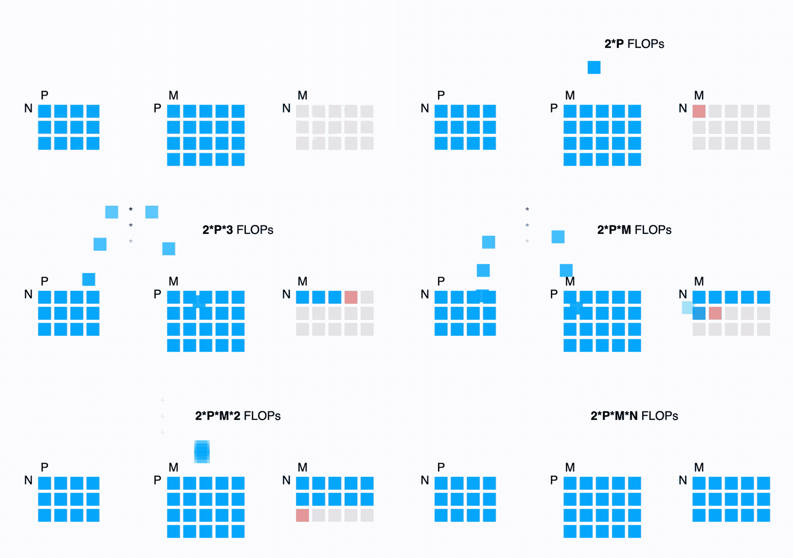
- A dot product of $$x \cdot y$$ requires $$P$$ adds and multiplies, or $$2P$$ floating-point operations total.
- A matrix-vector product $$Ax$$ does $$N$$ dot-products along the rows of $$A$$, for $$2NP$$ FLOPs.
- A matrix-matrix product $$AB$$ does a matrix-vector product for each of the $$M$$ columns of $$B$$, for $$2NPM$$ FLOPs total.
- In general, if we have two higher-dimensional arrays $$C$$ and $$D$$, where some dimensions are CONTRACTING and some are BATCHING (e.g. $$C[\blue{GH}IJ\red{KL}], D[\blue{GH}MN\red{KL}]$$), then the FLOPs cost of this contraction is two times the product of all of the $$C$$ and $$D$$ dimensions where the batch and contraction dimensions are only counted once (e.g. $$2\blue{GH}IJMN\red{KL}$$). Note that a dimension is only batching if it occurs in both multiplicands. (Note also that the factor of 2 won’t apply if there are no contracting dimensions and this is just an elementwise product.) (Contracting dimensions are axes that are summed over during the operation (they appear in both inputs but not in the output), like the inner dimension in a matrix multiply. Batching dimensions are shared axes that appear in both inputs and are carried unchanged to the output; they index independent subproblems and aren’t multiplied together in FLOP counts. In einsum terms: labels present on both inputs and the output are batching; labels present on both inputs but absent from the output are contracting.)
- 一次点积 $$x \cdot y$$ 需要 $$P$$ 次加法和乘法,总共是 $$2P$$ 次浮点运算。
- 矩阵-向量乘法 $$Ax$$ 会沿 $$A$$ 的各行做 $$N$$ 次点积,共 $$2NP$$ 次 FLOPs。
- 矩阵-矩阵乘法 $$AB$$ 会为 $$B$$ 的 $$M$$ 列各做一次矩阵-向量乘法,总共 $$2NPM$$ 次 FLOPs。
- 一般地,如果有两个更高维的数组 $$C$$ 和 $$D$$,其中一些维度是 CONTRACTING(收缩)、另一些是 BATCHING(批),例如 $$C[\blue{GH}IJ\red{KL}], D[\blue{GH}MN\red{KL}]$$,那么这次收缩的 FLOPs 代价等于:把 $$C$$ 和 $$D$$ 所有维度乘起来、其中批维度和收缩维度各只算一次,再乘以 2(例如 $$2\blue{GH}IJMN\red{KL}$$)。注意,一个维度只有在两个乘数里都出现时才算批维度。(还要注意,如果没有收缩维度、这只是一次逐元素相乘,那就不用乘 2。)(收缩维度是运算过程中被求和的轴(它们出现在两个输入里、但不出现在输出里),就像矩阵乘法里的内层维度。批维度是两个输入共享、并原样带到输出的轴;它们索引的是彼此独立的子问题,在 FLOPs 计数里不会相乘。用 einsum 的话说:两个输入和输出里都有的标签是批维度;两个输入里都有、但输出里没有的标签是收缩维度。)
$$ \begin{array}{ccc} \textrm{Operation} & \textrm{FLOPs} & \textrm{Data} \\ \hline x \cdot y & 2P & 2P \\ A x & 2NP & NP + P \\ AB & 2NPM & NP + PM \\ [c_0,...,c_N] \cdot [d_0,...,d_N] & 2 \prod c_i \times \prod_{\substack{d_j \notin \blue{BATCH} \\ d_j \notin \red{CONTRACT}}} d_j & \prod c_i + \prod d_j \\ \hline \end{array} $$
Make note of the fact that for a matrix-matrix multiply, the compute scales cubically $$O(N^3)$$ while the data transfer only scales quadratically $$O(N^2)$$ — this means that as we scale up our matmul size, it becomes easier to hit the compute-saturated limit. This is extremely unusual, and explains in large part why we use architectures dominated by matrix multiplication — they’re amenable to being scaled!
注意,对矩阵-矩阵乘法来说,计算量按三次方增长 $$O(N^3)$$,而数据传输量只按二次方增长 $$O(N^2)$$——这意味着随着矩阵乘法规模变大,我们反而更容易打到算力饱和的极限。这极其罕见,也在很大程度上解释了为什么我们用的架构都由矩阵乘法主导——因为它们天生适合被扩展!
Forward and reverse FLOPs
前向与反向 FLOPs
During training, we don’t particularly care about the result of a given matrix multiply; we really care about its derivative. It turns out that calculating that derivative costs about 3x more than just doing the matmul itself.
训练时我们并不特别关心某次矩阵乘法的结果,真正关心的是它的导数。而算这个导数的代价,大约是直接做那次矩阵乘法的 3 倍。
If we imagine B is just one matrix in a larger network and A are our input activations with C = A B, the derivative of the loss L with respect to B is given by the chain rule:
想象 B 只是更大网络里的一个矩阵,A 是我们的输入激活,C = A B,那么损失 L 对 B 的导数由链式法则给出:
$$\frac{\partial L}{\partial B} = \frac{\partial L}{\partial C}\frac{\partial C}{\partial B} = A^T \left(\frac{\partial L}{\partial C}\right)$$
which requires $2NPM$ FLOPs to compute (since it contracts over the $N$ dimension). Likewise, the derivative of the loss with respect to A is
计算它需要 $2NPM$ 次 FLOPs(因为它沿 $N$ 维度收缩)。同样地,损失对 A 的导数是
$$\frac{\partial L}{\partial A} = \frac{\partial L}{\partial C}\frac{\partial C}{\partial A} = \left(\frac{\partial L}{\partial C}\right) B^T$$
which is again $2NPM$ FLOPs since dL/dC is a matrix of size $$[N, M]$$. While this quantity isn’t the derivative w.r.t. a parameter, it’s used to compute derivatives for previous layers of the network (e.g. just as dL/dC is used to compute dL/dB above).
由于 dL/dC 是一个大小为 $$[N, M]$$ 的矩阵,这同样是 $2NPM$ 次 FLOPs。虽然它本身不是对参数的导数,但它会被用来求网络前面几层的导数(就像上面的 dL/dC 被用来求 dL/dB 一样)。
Adding these up, we see that during training, we have a total of 6NPM FLOPs, compared to 2NPM during inference: 2NPM in the forward pass, 4NPM in the backward pass. Since PM is the number of parameters in the matrix, this is the simplest form of the famous $$6 * \text{num parameters} * \text{num tokens}$$ approximation of Transformer FLOPs during training: each token requires $$6 * \text{num parameters}$$ FLOPs. We’ll show a more correct derivation below.
把这些加起来可以看到,训练时总共需要 6NPM 次 FLOPs,而推理时只需要 2NPM:前向 2NPM,反向 4NPM。由于 PM 就是矩阵里的参数量,这就得到了那条著名的近似:训练时 Transformer 的 FLOPs 约等于 $$6 * \text{参数数量} * \text{token 数量}$$,也就是每个 token 需要 $$6 * \text{参数数量}$$ 次 FLOPs。下面我们会给出更准确的推导。
Transformer Accounting
Transformer 账本
Transformers are the future. Well, they’re the present at least. Maybe a few years ago, they were one of many architectures. But today, it’s worth knowing pretty much every detail of the architecture. We won’t reintroduce the architecture, but this blog and the original Transformer paper may be helpful references.
Transformer 是未来。嗯,至少是现在。几年前它们还只是众多架构之一,但今天,把它的每个细节都搞清楚是值得的。我们不再重新介绍这个架构,不过这篇博客和原始的 Transformer 论文可以是很好的参考。
Here’s a basic diagram of the Transformer decoder architecture:
下面是 Transformer decoder 架构的示意图:
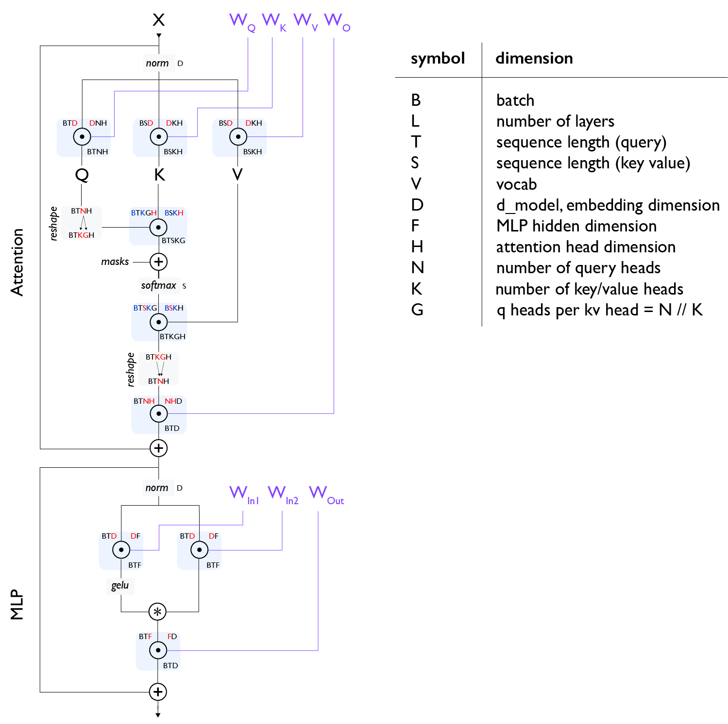
Note [gating einsum]: The diagram above uses a “gating einsum”[glu] where we split the up-projection matrix into two matrices ($W_\text{In1}$ and $W_\text{In2}$ above) whose outputs are elementwise multiplied as a kind of “gating function”. Not all LLMs use this, so you will sometimes see a single $W_\text{In}$ matrix and a total MLP parameter count of 2DF instead of 3DF. Typically in this case, D and F will be scaled up to keep the parameter count the same as the 3 matrix case. With that said, some form of gating einsum is used by LLaMA, DeepSeek, and many other models.
注 [gating einsum]:上图用的是「gating einsum」[glu],也就是把上投影矩阵拆成两个矩阵(上图的 $W_\text{In1}$ 和 $W_\text{In2}$),它们的输出做逐元素相乘,起到一种「门控函数」的作用。并非所有 LLM 都用它,所以你有时会看到单个 $W_\text{In}$ 矩阵,此时 MLP 总参数量是 2DF 而不是 3DF。这种情况下,D 和 F 通常会被放大,让参数量和三矩阵版本保持一致。话说回来,LLaMA、DeepSeek 等很多模型都用了某种形式的 gating einsum。
Note 2 [MHA attention]: With self-attention, T and S are the same but for cross-attention they may be different. With vanilla Multi-Head Attention (MHA), N and K are the same while for Multi-Query Attention (MQA)[mqa] K=1 and for Grouped MQA (GMQA)[gmqa], K merely has to divide N.
注 2 [MHA 注意力]:在自注意力里 T 和 S 相同,但在交叉注意力里它们可能不同。在朴素的多头注意力(MHA)里 N 和 K 相同,而在 Multi-Query Attention(MQA)[mqa] 里 K=1,在 Grouped MQA(GMQA)[gmqa] 里 K 只需能整除 N。
Note 3 [pre-norm vs. post-norm]: The above diagram shows what is known as a “pre-norm” architecture in which the norm occurs before the residual connection, usually as x + attn(norm(x)). Models like LLaMA-3 use this today. The original Transformer paper used a “post-norm” architecture in which the layernorm occurs after the residual connection, i.e. norm(x + attn(x)).
注 3 [pre-norm 与 post-norm]: 上图展示的是所谓的「pre-norm」架构,归一化发生在残差连接之前,通常是 x + attn(norm(x))。LLaMA-3 这类模型现在就用这个。原始 Transformer 论文用的是「post-norm」,layernorm 发生在残差连接之后,即 norm(x + attn(x))。
Global FLOPs and Params Calculation
全局 FLOPs 与参数量计算
Let’s calculate the per-layer FLOPs of a Transformer (so we can avoid having to stick factors of L everywhere). Note that the training FLOPs below are almost always 3x the inference FLOPs, so you can divide any total by 3 to get the cost of just the forward pass.
我们来算一下 Transformer 单层的 FLOPs(这样就不必处处都挂一个 L 因子)。注意下面训练时的 FLOPs 几乎总是推理时的 3 倍,所以任何总量除以 3 就是纯前向的代价。
MLPs
MLP
The MLPs of a Transformer typically consist of 2 input matmuls that are element-wise combined and a single output matmul:
Transformer 的 MLP 通常由两个输入矩阵乘法(逐元素合并)和一个输出矩阵乘法组成:
$$ \begin{array}{ccc} \textrm{operation} & \textrm{train FLOPs} & \textrm{params} \\ \hline \\ A[B,T,\red{D}] \cdot W_{in1}[\red{D}, F] & 6BTDF & DF \\[10pt] A[B,T,\red{D}] \cdot W_{in2}[\red{D}, F] & 6BTDF & DF \\[10pt] \sigma\left(A_{in1}\right)[B,T, F] * A_{in2}[B,T, F] & \gray{O(BTF)} \\[10pt] A[B,T,\red{F}] \cdot W_{out}[\red{F}, D] & 6BTDF & DF \\[10pt] \hline \\ & \approx 18BTDF & 3DF \end{array} $$
Attention
注意力
For the generic grouped-query attention case with different Q and KV head numbers, let us assume equal head dimension H for Q,K,V projections, and estimate the cost of the QKVO matmuls:
对 Q 头和 KV 头数量不同的通用 group-query attention,我们假设 Q、K、V 投影的头维度 H 相同,并估算 QKVO 这几个矩阵乘法的代价:
$$ \begin{array}{ccc} \textrm{operation} & \textrm{train FLOPs} & \textrm{params} \\ \hline \\ A[B,T,\red{D}] \cdot W_{Q}[\red{D}, N, H] & 6BTDNH & DNH \\[10pt] A[B,T,\red{D}] \cdot W_{K}[\red{D}, K, H] & 6BTDKH & DKH \\[10pt] A[B,T,\red{D}] \cdot W_{V}[\red{D}, K, H] & 6BTDKH & DKH \\[10pt] A[B,T,\red{N}, \red{H}] \cdot W_{O}[\red{N}, \red{H}, D] & 6BTDNH & DNH \\[10pt] \hline \\ & 12BTD(N+K)H & 2D(N+K)H \end{array} $$
The dot-product attention operation is more subtle, effectively being a $$TH \cdot HS$$ matmul batched over the $$B$$, $$K$$ dimensions, a softmax, and a $$TS \cdot SH$$ matmul again batched over the $$B$$, $$K$$ dimensions. We highlight the batched dims in blue:
点积注意力要更微妙一些:它实际上是一次 $$TH \cdot HS$$ 矩阵乘法(在 $$B$$、$$K$$ 维度上批处理)、一次 softmax,再加一次 $$TS \cdot SH$$ 矩阵乘法(同样在 $$B$$、$$K$$ 维度上批处理)。我们用蓝色标出批维度:
$$ \begin{array}{cc} \textrm{operation} & \textrm{train FLOPs} \\ \hline \\[3pt] Q[\blue{B}, T, \blue{K}, G, \red{H}] \cdot K[\blue{B}, S, \blue{K}, \red{H}] & 6BTSKGH = 6BTSNH \\[3pt] \textrm{softmax}_S \;\; L[B, T, S, K, G] & \gray{O(BTSKG) = O(BTSN)} \\[3pt] S[\blue{B}, T, \red{S}, \blue{K}, G] \cdot V[\blue{B}, \red{S}, \blue{K}, H] & 6BTSKGH = 6BTSNH \\[3pt] \hline \\ & \approx 12BTSNH = 12BT^2NH \\ \end{array} $$
Note [causal masking]: Most recent transformers use a causal mask as opposed to full bidirectional attention. In this case the useful FLOPs of the dot product operations are reduced by half. To achieve this reduction in practice we need to make use of an attention kernel, rather than a naive einsum.
注 [causal masking]:最近大多数 Transformer 用的都是 causal mask,而不是完整的双向注意力。这种情况下,点积运算的有效 FLOPs 会减半。要在实践中拿到这个减半,我们得用 attention kernel,而不是朴素的 einsum。
Other Operations
其他运算
There are several other operations happening in a Transformer. Layernorms are comparatively cheap and can be ignored for first-order cost estimates. Note that each layer typically has two of them (one before attention and one before the MLP). There is also the final enormous (though not per-layer) unembedding matrix multiply.
Transformer 里还有若干其他运算。Layernorm 相对便宜,做一阶代价估算时可以忽略。注意每层通常有两个 layernorm(一个在注意力之前,一个在 MLP 之前)。另外还有一个巨大的(虽然不属于单层)最终 unembedding 矩阵乘法。
$$ \begin{array}{ccc} \textsf{operation} & \textsf{train FLOPs} & \textsf{params} \\ \hline \\ 2 \times \textrm{layernorm}_D \;\; A[B,T,\red{D}] & \gray{O\left(BTD\right)} & \gray{2D} \\[10pt] A[B,T,\red{D}] \cdot W_{unembed}[\red{D}, V] & 6BTDV & DV \\ \end{array} $$
General rule of thumb for Transformer FLOPs
Transformer FLOPs 的经验法则
If we neglect the cost of dot-product attention (which is reasonable for shorter-context training), then the total FLOPs across all layers is
如果忽略点积注意力的代价(在上下文不太长的训练里这是合理的),那么所有层加起来的总 FLOPs 是
$$ \begin{align*} (18BTDF + 12BTD(N+K)H)L = 6 *BT * (3DF + 2D(N+K)H)L \\ = 6 * \textrm{num tokens} * \textrm{parameter count} \end{align*} $$
This leads to a famous rule of thumb for estimating dense Transformer FLOP count, ignoring the attention FLOPs. (Unembedding is another simple matmul with $6BTDV$ FLOPs and $DV$ params, and follows the same rule of thumb.)
这就引出了那条估算稠密 Transformer FLOPs 的著名经验法则(忽略注意力部分)。(Unembedding 是另一个简单的矩阵乘法,$$6BTDV$$ 次 FLOPs、$$DV$$ 个参数,同样遵循这条法则。)
Fractional cost of attention with context length
注意力代价随上下文长度的占比
If we do account for dot-product attention above and assume $$F=4D$$, $$D=NH$$ (as is typical) and $$N=K$$, the ratio of dot-product attention FLOPs to all matmul FLOPs (including the attention projections) is:
如果认真计入上面的点积注意力,并假设 $$F=4D$$、$$D=NH$$(这是典型情况)以及 $$N=K$$,那么点积注意力的 FLOPs 与全部矩阵乘法 FLOPs(含注意力投影)之比是:
$$\small{\frac{\textrm{attention FLOPs}}{\textrm{matmul FLOPs}} = \frac{12BT^2NH}{18BTDF + 24BTDNH} = \frac{12BT^2D}{4*18 BTD^2 + 24 BTD^2} = \frac{12BT^2D}{96 BTD^2} = \frac{T}{8D}}$$
The upshot is that dot-product attention FLOPs only become dominant during training once T>8D. For D ~ 8k, this would be ~64K tokens. This makes some sense, since it means as the MLP size increases, the attention FLOPs become less critical. For large models, the quadratic cost of attention is not actually a huge obstacle to longer-context training. However, for smaller models, e.g. Gemma-27B with D=4608, attention becomes dominant around 37k sequence lengths. (Note that some modern OSS models introduce local attention or other optimizations that reduce the cost of attention and change this roofline.) Flash Attention also helps alleviate the cost of long-context, which we discuss briefly in Appendix A.
结论是:训练时,只有当 T>8D 之后,点积注意力的 FLOPs 才会占主导。 对 D ~ 8k 来说,这大约是 64K 个 token。这其实说得通:MLP 越大,注意力的 FLOPs 就越不关键。对大模型来说,注意力的二次代价并不是长上下文训练的什么大障碍。但对小模型就不是了,比如 D=4608 的 Gemma-27B,注意力在约 37k 序列长度时就开始占主导。(注意一些现代开源模型引入了 local attention 或其他优化,降低了注意力的代价,也就改变了这条 roofline。)Flash Attention 也有助于缓解长上下文的代价,我们在附录 A 里简单讨论。
Miscellaneous Math
零散数学
Sparsity and Mixture-of-Experts
稀疏性与混合专家
We’d be remiss not to briefly discuss Mixture of Experts (MoE) models[moe], which replace the single dense MLP blocks in a standard Transformer with a set of independent MLPs that can be dynamically routed between. To a first approximation, an MoE is just a normal dense model with E MLP blocks per layer, instead of just one. Each token activates $k$ of these experts, typically $k \ll E$. The ratio $E / k$ is called the sparsity and is usually between 8 and 64 (e.g. DeepSeek v3 has effectively $k=8$, $E=256$). This increases the parameter count by $O(E)$, while multiplying the total number of activated parameters per token by $k$, compared with the dense version.
不简单聊聊混合专家(MoE)模型[moe] 就太失职了:它把标准 Transformer 里单个稠密 MLP 块换成一组彼此独立的 MLP,可以在它们之间动态路由。粗略地说,MoE 就是一个普通稠密模型,只是每层有 E 个 MLP 块,而不是一个。每个 token 激活其中 $k$ 个专家,通常 $k \ll E$。比值 $E / k$ 称为稀疏度,通常在 8 到 64 之间(例如 DeepSeek v3 实际上 $k=8$、$E=256$)。相比稠密版本,这让参数量增加 $O(E)$,同时把每个 token 激活的参数量乘以 $k$。
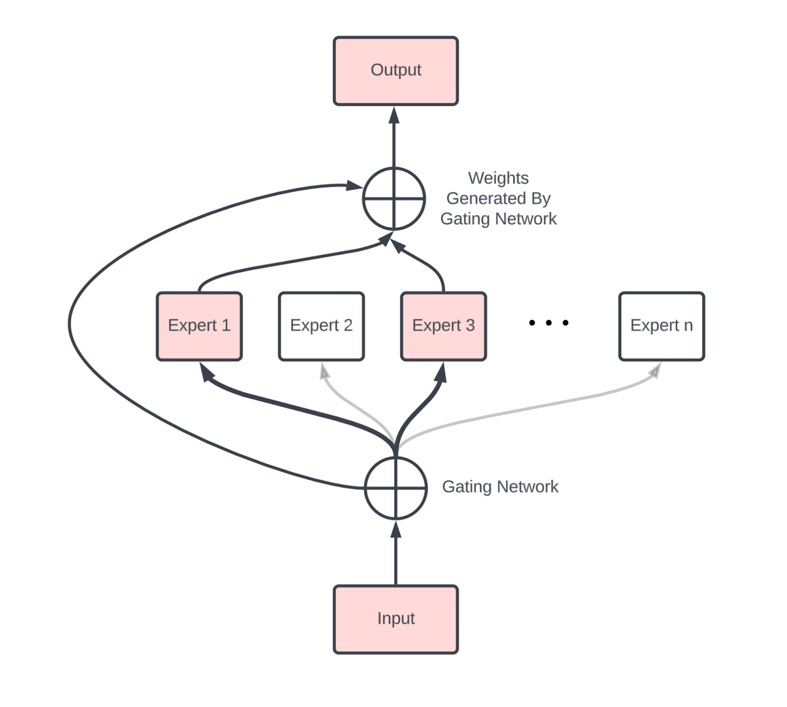
Compared to a dense model, an MoE introduces new comms, primarily two AllToAlls (one before and one after the MoE block) that route tokens to the correct expert and bring them back to their home device. (Technically, this only happens if we are data or sequence sharded along the same axis as our experts.) However, as we saw in the previous section, the cost of each AllToAll is only 1/4 that of a comparable AllGather along a single axis (for a bidirectional ring).
相比稠密模型,MoE 引入了新的通信,主要是两次 AllToAll(一次在 MoE 块之前、一次在之后),把 token 路由到正确的专家、再送回它们原来的设备。(严格说,只有当我们沿专家所在的同一个轴做数据并行或序列并行时才会这样。)不过,如上一节所见,在双向环上,一次 AllToAll 的代价只有单轴 AllGather 的 1/4。
Gradient checkpointing
梯度检查点(Gradient checkpointing)
Backpropagation as an algorithm trades compute for memory. Instead of a backward pass requiring $$O(n_\text{layers}^2)$$ FLOPs, it requires $$O(n_\text{layers})$$ memory, saving all intermediate activations generated during the forward pass. While this is better than quadratic compute, it’s incredibly expensive memory-wise: a model with $$B * T=4M$$ (4M total tokens per batch), L=64, and D=8192 that avoids all unnecessary backward pass compute would have to save roughly $$2 * 20 * B * T * D * L = 84TB$$ of activations in bfloat16. The 20 comes from (roughly) counting every intermediate node in the Transformer diagram above, since e.g.
反向传播这个算法是在用计算换内存。反向传播不再需要 $$O(n_\text{layers}^2)$$ 次 FLOPs,而是只需要 $$O(n_\text{layers})$$ 的内存,代价是把前向过程中产生的所有中间激活都存下来。虽然这比二次方的计算要好,但在内存上极其昂贵:一个 $$B * T=4M$$(每批共 4M 个 token)、L=64、D=8192 的模型,如果完全不做多余的反向计算,就得在 bfloat16 下存下大约 $$2 * 20 * B * T * D * L = 84TB$$ 的激活。这里的 20 大致来自把上面 Transformer 示意图里的每个中间节点都数了一遍,因为例如
$$f(x) = \exp(g(x))$$
$$\frac{df}{dx} = \exp(g(x)) \cdot \frac{dg}{dx}$$
so to avoid recomputing we need to save $$g(x)$$ and $$\exp(g(x))$$ from the forward pass. To avoid saving this much memory, we can choose to only save some fraction of the intermediate activations. Here are a few strategies we use.
所以为了避免重算,我们需要在前向里存下 $$g(x)$$ 和 $$\exp(g(x))$$。为了不存这么多内存,我们可以选择只保存一部分中间激活。下面是我们会用的一些策略。
- Block remat: only save the input to each layer. This is the most aggressive method we use and only saves 1 checkpoint per layer, meaning we’d only save 4.2TB in the example above. This forces us to repeat essentially all forward pass FLOPs in the backward pass, meaning we increase our FLOPs from $$6 \cdot \text{num params} \cdot \text{num tokens}$$ to roughly $$8 \cdot \text{num params} \cdot \text{num tokens}$$.
- Big matmuls only: another simple policy is to only save the outputs of large matmuls. This lets us avoid recomputing any large matmuls during the backward pass, but still makes us recompute other activation functions and parts of attention. This reduces the 20 per layer above to closer to 7 per layer.
- Block remat:只保存每层的输入。这是我们最激进的做法,每层只存 1 个检查点,上面那个例子里就只需要 4.2TB。代价是反向传播时几乎要把整个前向的 FLOPs 重做一遍,也就是把 FLOPs 从 $$6 \cdot \text{num params} \cdot \text{num tokens}$$ 提高到大约 $$8 \cdot \text{num params} \cdot \text{num tokens}$$。
- 只存大矩阵乘法:另一个简单策略是只保存大矩阵乘法的输出。这样反向传播时不需要重算任何大矩阵乘法,但仍要重算其他激活函数和注意力的一部分。这把上面每层的 20 降到接近每层 7。
This is by no means comprehensive. When using JAX, these are typically controlled by jax.remat/jax.checkpoint (you can read more here).
这远非全部做法。用 JAX 时,这些通常由 jax.remat/jax.checkpoint 控制(更多内容见这里)。
Key-Value (KV) caching
Key-Value(KV)缓存
As we’ll see in Section 7, LLM inference has two key parts, prefill and generation.
我们会在第 7 节看到,LLM 推理有两个关键部分:prefill 和 generation。
- Prefill processes a long prompt and saves its attention activations in a Key-Value Cache (KV Cache) for use in generation, specifically the key-value projections in the attention block.
- Generation batches several of these KV caches together and samples tokens from each of them.
- Prefill 处理一段很长的 prompt,并把它的注意力激活存进 Key-Value Cache(KV Cache)供 generation 使用,具体说是注意力块里的 key-value 投影。
- Generation 把若干个这样的 KV cache 批在一起,从每一个里采样 token。
Each KV cache is then effectively an array of size $[2, S, L, K, H]$ where the 2 accounts for the keys and values. This is quite large! The total size of the Key-Value cache in int8 is $2SLKH$. For a moderately sized model with 8k context length, 64 layers, and $KH = NH = D = 8192$, this is $2 \cdot 8192 \cdot 64 \cdot 8192 = 8\text{GiB}$. You can see why we would want to use GMQA with $K \ll N$.
于是每个 KV cache 实际上是一个大小为 $[2, S, L, K, H]$ 的数组,其中 2 是因为 key 和 value 各一份。这相当大!int8 下 Key-Value cache 的总大小是 $2SLKH$。对一个中等规模的模型,上下文长度 8k、64 层、$KH = NH = D = 8192$,这就是 $2 \cdot 8192 \cdot 64 \cdot 8192 = 8\text{GiB}$。你能明白为什么我们会想用 $K \ll N$ 的 GMQA 了。
What Should You Take Away from this Section?
这一节你应该带走什么?
- The overall parameters and FLOPs of a Transformer are fairly easy to calculate, and are summarized here, assuming MHA (with batch size B, vocab size V, a sequence of length T, D=dmodel, and F=dff):
- Transformer 的整体参数量和 FLOPs 相当容易算,假设用 MHA(batch size 为 B、词表大小为 V、序列长度为 T、D=dmodel、F=dff),可以汇总成下面这张表:
| Component | Params per layer | Training FLOPs per layer |
|---|---|---|
| MLP | 3DF | 18BTDF |
| Attention | 4DNH | 24BTDNH + 12BT2NH |
| Other | 2D | BTD |
| Vocab | DV (total, not per-layer) | 12BTDV |
- The parameter count of the MLP block dominates the total parameter count and the MLP block also dominates the FLOPs budget as long as the sequence length $T < 8D$.
- The total FLOPs budget during training is well approximated by $$6 \cdot \text{num\_params} \cdot \text{num\_tokens}$$ for reasonable context lengths.
- During inference, our KV caches are roughly $$2 \cdot S \cdot L \cdot K \cdot H$$ per cache (where K is the number of KV heads), although architectural modifications can often reduce this.
- MLP 块的参数量在整个参数量里占主导;只要序列长度 $T < 8D$,MLP 块在 FLOPs 预算里同样占主导。
- 在合理的上下文长度下,训练时的总 FLOPs 预算可以很好地用 $$6 \cdot \text{num\_params} \cdot \text{num\_tokens}$$ 近似。
- 推理时,每个 KV cache 大约是 $$2 \cdot S \cdot L \cdot K \cdot H$$(K 是 KV 头数),不过架构上的改动往往能把它降下来。
A Few Problems to Work
几道练习题
Question 1: How many parameters does a model with $D=4096$, $F=4 \cdot D$, $V=32,000$, and $L=64$ have? What fraction of these are attention parameters? How large are our KV caches per token? You can assume $N\cdot H=D$ and multi-head attention with int8 KVs.
第 1 题: 一个 $D=4096$、$F=4 \cdot D$、$V=32,000$、$L=64$ 的模型有多少参数?其中注意力参数占多大比例?每个 token 的 KV cache 有多大?可以假设 $N\cdot H=D$,用多头注意力,KV 用 int8。
Click here for the answer.
点这里看答案。
- The total parameters is roughly $$L \cdot (3DF + 4DNH + 2D) + 2DV$$ (counting the two layernorms per layer). For the given numbers, this is $$64 \cdot (3 \cdot 4e3 \cdot 16e3 + 4 \cdot 4e3 \cdot 4e3 + 2 \cdot 4e3) + 2 \cdot 4e3 \cdot 32e3 = 16e9$$, or 16B parameters.
- The ratio of attention parameters to total parameters in general is $$4DNH / (4DNH + 3DF) = 4D^2 / (4D^2 + 12D^2) = 1/4$$. This means roughly 1/4 of the parameters are used in attention.
- Per token, our KV caches are $$2 \cdot L \cdot N \cdot H = 2 \cdot 64 \cdot 4096$$ in int8, which is
512 KiB / token.
- 总参数量大致是 $$L \cdot (3DF + 4DNH + 2D) + 2DV$$(把每层两个 layernorm 也算上)。代入给定数字:$$64 \cdot (3 \cdot 4e3 \cdot 16e3 + 4 \cdot 4e3 \cdot 4e3 + 2 \cdot 4e3) + 2 \cdot 4e3 \cdot 32e3 = 16e9$$,也就是 16B 参数。
- 一般地,注意力参数占总参数的比例是 $$4DNH / (4DNH + 3DF) = 4D^2 / (4D^2 + 12D^2) = 1/4$$。也就是说大约 1/4 的参数用在注意力上。
- 每个 token 的 KV cache 是 $$2 \cdot L \cdot N \cdot H = 2 \cdot 64 \cdot 4096$$(int8),即
512 KiB / token。
Question 2: How many total FLOPs are required to perform A[BX, DY] *D W[DY, F] on {'X': 4, 'Y': 8, 'Z': 4}? How many FLOPs are performed by each TPU?
第 2 题: 在 {'X': 4, 'Y': 8, 'Z': 4} 上执行 A[BX, DY] *D W[DY, F] 总共需要多少 FLOPs?每块 TPU 做多少 FLOPs?
Click here for the answer.
点这里看答案。
The total “theoretical” FLOPs of the operation is $$2 \cdot B \cdot D \cdot F$$. However, because the computation isn’t sharded across the Z dimension, we’re actually doing Z extra FLOPs, meaning $$2 \cdot B \cdot D \cdot F \cdot Z$$ total FLOPs. Since the computation is sharded across the other dimensions, the total per-device is roughly $$2 \cdot B \cdot D \cdot F / (X \cdot Y)$$.
这次运算「理论上」的总 FLOPs 是 $$2 \cdot B \cdot D \cdot F$$。但由于计算没有在 Z 维度上分片,我们实际上多做了 Z 倍的 FLOPs,也就是总共 $$2 \cdot B \cdot D \cdot F \cdot Z$$ 次 FLOPs。又因为计算在其他维度上是分片的,每块设备大约是 $$2 \cdot B \cdot D \cdot F / (X \cdot Y)$$。
Question 3: How many FLOPs are involved in performing $A[I,J,K,L] * B[I,J,M,N,O] \rightarrow C[K,L,M,N,O]$?
第 3 题: 执行 $A[I,J,K,L] * B[I,J,M,N,O] \rightarrow C[K,L,M,N,O]$ 涉及多少 FLOPs?
Click here for the answer.
点这里看答案。
Following the rule above, we have I and J as contracting dimensions and K, L, M, N, and O as non-contracting dimensions. We have no “batching dimensions”, so this is just $$2 \cdot I \cdot J \cdot K \cdot L \cdot M \cdot N \cdot O$$, the product of all the axes. If we had a shared axis, it would only be counted once.
按上面的规则,I 和 J 是收缩维度,K、L、M、N、O 是非收缩维度。这里没有「批维度」,所以就是 $$2 \cdot I \cdot J \cdot K \cdot L \cdot M \cdot N \cdot O$$,也就是所有轴的乘积。如果有共享的轴,它只会被算一次。
Question 4: What is the arithmetic intensity of grouped multi-query attention (ignoring the Q/K/V/O projections)? Give the answer as a function of the Q and KV sequence lengths T and S and the multi-query factor G. At what context length is attention FLOPs-bound? Given the HBM bandwidth of our TPUs, plot the effective relative cost of attention to the FFW block as the context length grows. Hint: assume we’re using an efficient attention implementation that doesn’t do any unnecessary reads/writes. Consider both the limits where T = S and T << S.
第 4 题: grouped multi-query attention 的算术强度是多少(忽略 Q/K/V/O 投影)?答案写成 Q 与 KV 序列长度 T 和 S、以及 multi-query 因子 G 的函数。 上下文多长时注意力是计算受限的?给定我们 TPU 的 HBM 带宽,画出随上下文长度增长、注意力相对 FFW 块的有效代价曲线。提示:假设我们用的是高效注意力实现,不做任何多余的读写。分别考虑 T = S 和 T << S 两个极限。
Click here for the answer.
点这里看答案。
Self-attention requires loading the $$Q$$, $$K$$, and $$V$$ activations, then computing $$\text{softmax}(Q \cdot K) \cdot V$$, then writing the result back to HBM. This will be done with Flash Attention so there are some caveats to this math, but basically in bf16 self-attention performs
自注意力需要加载 $$Q$$、$$K$$、$$V$$ 激活,然后计算 $$\text{softmax}(Q \cdot K) \cdot V$$,再把结果写回 HBM。实际会用 Flash Attention 来做,所以这个计算有些附加说明,但基本上 bf16 下自注意力做的事是
$$\text{Q[B,T,N,H]} \rightarrow_\text{reshape} \text{Q[B, T, K, G, H]} \cdot \text{K[B, S, K, H]} \rightarrow \text{O[B, T, S, K, G]}$$
$$U=\text{softmax}_S(\text{O[B, T, S, K, G]})$$
$$\text{U[B, T, S, K, G]} \cdot \text{V[B, S, K, H]} \rightarrow \text{X[B, T, K, G, H]}$$
So our total bytes is $$2 * \text{sizeof}(Q) + 2 * \text{sizeof(K or V)} = 4BTNH + 4BSKH = 4BHK * (TG + S)$$, total FLOPs is $$4BTSNH + O(BTSN)$$ and the arithmetic intensity is $$4BTSKGH / (4BHK * (TG + S))$$.
所以总字节数是 $$2 * \text{sizeof}(Q) + 2 * \text{sizeof(K or V)} = 4BTNH + 4BSKH = 4BHK * (TG + S)$$,总 FLOPs 是 $$4BTSNH + O(BTSN)$$,算术强度是 $$4BTSKGH / (4BHK * (TG + S))$$。
So basically, during prefill we have $$S=T$$ so we have an arithmetic intensity of $$4BT^2KGH / 4BHKT \cdot (G+1) = TG/(G + 1) = O(T)$$. During generation, $$T=1$$ so we have $$4BSKGH / (4BHK \cdot (G + S)) = SG / (G + S) \rightarrow G$$ assuming $$S$$ is very large. Depending on how you interpret the question, during prefill or training self-attention is compute-bound at S=240 assuming no sequence sharding. During generation, we are never compute-bound because $$G$$ is small. Nonetheless, you can see that increasing $$G$$ leads to us being closer to compute-bound.
所以在 prefill 阶段我们有 $$S=T$$,算术强度是 $$4BT^2KGH / 4BHKT \cdot (G+1) = TG/(G + 1) = O(T)$$。在 generation 阶段 $$T=1$$,于是得到 $$4BSKGH / (4BHK \cdot (G + S)) = SG / (G + S) \rightarrow G$$(假设 $$S$$ 非常大)。取决于你怎么理解这个问题,在没有序列分片的前提下,prefill 或训练时自注意力在 S=240 时变成计算受限。generation 阶段则永远不会计算受限,因为 $$G$$ 很小。尽管如此,你可以看到增大 $$G$$ 会让我们更接近计算受限。
Question 5: At what sequence length are self-attention FLOPs equal to the QKVO projection FLOPs?
第 5 题: 序列多长时,自注意力的 FLOPs 等于 QKVO 投影的 FLOPs?
Click here for the answer.
点这里看答案。
This is purely a question of when $$24BTDNH = 12BT^2NH$$. Simplifying we get $$2D = T$$, so e.g. for $$D=4096$$, this is $$8192$$. This tells us that for most reasonable context lengths, matmul FLOPs are greater.
纯粹就是问什么时候 $$24BTDNH = 12BT^2NH$$。化简得到 $$2D = T$$,所以例如 $$D=4096$$ 时是 $$8192$$。这说明在大多数合理的上下文长度下,矩阵乘法的 FLOPs 更大。
Question 6: Say we only save the output of each of the 7 main matmuls in a Transformer layer during our forward pass (Q, K, V, O + the three FFW matrices). How many extra FLOPs do we need to “rematerialize” during the backward pass?
第 6 题: 假设前向传播时我们只保存 Transformer 每一层里 7 个主要矩阵乘法的输出(Q、K、V、O + 三个 FFW 矩阵)。反向传播时需要多花多少 FLOPs 来「重新物化」?
Click here for the answer.
点这里看答案。
Saving only the seven matmul outputs (Q, K, V, O, W₁, W₂, W₃) means the backward pass must recompute the two attention matmuls
只保存七个矩阵乘法输出(Q、K、V、O、W₁、W₂、W₃)意味着反向传播必须重算两次注意力矩阵乘法
$$QK^{\top} \quad\text{and}\quad \operatorname{softmax}(QK^{\top})V$$
in order to obtain $\frac{\partial L}{\partial W_\text{O}}$.
才能得到 $\frac{\partial L}{\partial W_\text{O}}$。
Each is a $T \times T$ matmul batched over $B$ sequences and $N$ heads, so the additional FLOPs are
两者都是 $T \times T$ 的矩阵乘法,在 $B$ 个序列和 $N$ 个头之上批处理,所以额外的 FLOPs 是
$$4 \; B \, T^{2} \, N \, H.$$
Other recomputed operations are:
其他需要重算的运算还有:
- $O(BTD)$ for $\frac{\partial L}{\partial W_\text{In1}}$ and $\frac{\partial L}{\partial W_\text{In2}}$.
- And $O(BTF)$ for $\frac{\partial L}{\partial W_\text{Out}}$.
- $\frac{\partial L}{\partial W_\text{In1}}$ 和 $\frac{\partial L}{\partial W_\text{In2}}$ 的 $O(BTD)$。
- 以及 $\frac{\partial L}{\partial W_\text{Out}}$ 的 $O(BTF)$。
Question 7: DeepSeek v3 says it was trained for 2.79M H800 hours on 14.8T tokens (source). Given that it has 37B activated parameters, roughly what hardware utilization did they achieve? Hint: note that they used FP8 FLOPs without structured sparsity.
第 7 题: DeepSeek v3 说它用了 279 万 H800 小时、训练了 14.8T 个 token(来源)。考虑到它有 37B 激活参数,他们大致达到了多少硬件利用率?提示:注意他们用的是不带结构化稀疏的 FP8 FLOPs。
Click here for the answer.
点这里看答案。
From the spec sheet here, we find 3,026 TFLOPs/s of FP8 performance with sparsity, or typically half this (1.513e15 FLOPs/s) without sparsity. 2.79M H800 hours means 2.79e6 * 1.513e15 * 60 * 60 = 1.52e25 total FLOPs. Given the activated parameter count of 37B, this training run should have used about 6 * 37e9 * 14.8e12 = 3.3e24 FLOPs. That means the FLOPs utilization is about 3.3e24 / 1.52e25 = 21.7%.
从这份规格表可以看到,带稀疏时 FP8 性能是 3,026 TFLOPs/s,不带稀疏通常是它的一半(1.513e15 FLOPs/s)。279 万 H800 小时意味着 2.79e6 * 1.513e15 * 60 * 60 = 1.52e25 次 FLOPs。按 37B 激活参数量算,这次训练大约应该用掉 6 * 37e9 * 14.8e12 = 3.3e24 次 FLOPs。也就是说 FLOPs 利用率约为 3.3e24 / 1.52e25 = 21.7%。
Question 8: Mixture of Experts (MoE) models have $E$ copies of a standard dense MLP block, and each token activates $k$ of these experts. What batch size in tokens is required to be compute-bound for an MoE with weights in int8 on TPU v5e? For DeepSeek, which has 256 (routed) experts and $k=8$, what is this number?
第 8 题: 混合专家(MoE)模型有 $E$ 份标准稠密 MLP 块,每个 token 激活其中 $k$ 个专家。权重用 int8、在 TPU v5e 上时,要多大的 batch size(按 token 数)才能做到计算受限?对 DeepSeek 来说,它有 256 个(被路由的)专家、$k=8$,这个数字是多少?
Click here for the answer.
点这里看答案。
Because we have $E$ copies of each expert, in int8, for each weight matrix we need to load $E \cdot D \cdot F$ bytes. Because each token activates $k$ experts, for each weight matrix we have $2\cdot k \cdot B \cdot D \cdot F$ FLOPs. To be compute-bound with int8 weights and bfloat16 FLOPs, we need the arithmetic intensity (FLOPs per byte loaded) to exceed the TPU’s ~240 FLOPs/byte, which happens when $(2\cdot k \cdot BDF) / EDF > 240$ or $k \cdot B / E > 120$.
因为我们有 $E$ 份每个专家,int8 下每个权重矩阵都要加载 $E \cdot D \cdot F$ 字节。又因为每个 token 激活 $k$ 个专家,每个权重矩阵对应 $2\cdot k \cdot B \cdot D \cdot F$ 次 FLOPs。要在 int8 权重、bfloat16 FLOPs 下做到计算受限,算术强度(每加载一字节对应的 FLOPs)必须超过 TPU 的约 240 FLOPs/byte,即 $(2\cdot k \cdot BDF) / EDF > 240$,也就是 $k \cdot B / E > 120$。
Therefore, we need $B > 120 \cdot E / k$ to be compute-bound. For DeepSeek, this gives us $B > 120 \cdot 256 / 8 = 3840$. This is a remarkably large batch size at generation time.
因此要做到计算受限,需要 $B > 120 \cdot E / k$。对 DeepSeek 来说就是 $B > 120 \cdot 256 / 8 = 3840$。在生成阶段,这是一个相当惊人的 batch size。
That’s it for Part 4! For Part 5 (about scaling Transformer training), click here!
第 4 部分到此结束!第 5 部分(关于扩展 Transformer 训练)请点这里!
Appendix
附录
Appendix A: How does Flash Attention work?
附录 A:Flash Attention 是怎么工作的?
The traditional objection to scaling Transformers to very long context is that the attention FLOPs and memory usage scale quadratically with context length. While it’s true that the attention QK product has shape $[B, T, S, N]$ where B is the batch size, T and S are the Q and K sequence dims, and N is the number of heads, this claim comes with some serious caveats:
传统上反对把 Transformer 扩展到超长上下文的理由是:注意力 FLOPs 和内存占用随上下文长度二次增长。虽然注意力 QK 乘积的形状确实是 $[B, T, S, N]$(B 是 batch size,T 和 S 是 Q 和 K 的序列维度,N 是头数),但这个论断有几个重要的前提:
- As we noted earlier, even though this is quadratic, the attention FLOPs only dominate when $$T > 8 \cdot D$$, and during training the memory of a single attention matrix is small compared to all of the weights and activation checkpoints living in memory, especially when sharded.
- We don’t need to materialize the full attention matrix in order to compute attention! We can compute local sums and maxes and avoid ever materializing more than a small chunk of the array. While the total FLOPs is still quadratic, we drastically reduce memory pressure.
- 如我们前面所说,虽然它是二次的,但注意力 FLOPs 只有在 $$T > 8 \cdot D$$ 时才占主导;而且训练时单个注意力矩阵的内存,相比内存里所有能存的权重和激活检查点(尤其在分片之后)是很小的。
- 我们并不需要真的把完整的注意力矩阵物化出来才能算注意力!我们可以计算局部和与局部最大值,从而永远不需要物化超过一小块的数组。虽然总 FLOPs 仍是二次的,但内存压力大幅降低。
This second observation was first made by Rabe et al. 2021 and later in the Flash Attention paper (Dao et al. 2022). The basic idea is to compute the attention in chunks of K/V, where we compute the local softmax and some auxiliary statistics, then pass them on to the next chunk which combines them with its local chunk. Specifically, we compute
第二个观察最早由 Rabe 等人 2021 提出,后来出现在 Flash Attention 论文(Dao 等人 2022)里。基本思路是按 K/V 分块计算注意力:先算出局部 softmax 和一些辅助统计量,再传给下一块,与它本地的块合并。具体来说,我们计算
- M: The running max of $$q \cdot k$$ over the sequence dimension
- O: The running full attention softmax over the sequence dimension
- L: The running denominator $$\sum_i \exp(q \cdot k_i - \text{running max})$$
- M: $$q \cdot k$$ 沿序列维度的running max
- O: 沿序列维度的running完整注意力 softmax
- L: running 分母 $$\sum_i \exp(q \cdot k_i - \text{running max})$$
With these, we can compute the new max, the new running sum, and the new output with only a constant amount of memory. To give a sketchy description of how this works, attention is roughly this operation:
有了这些,我们只需要常数级内存就能算出新的最大值、新的累计和以及新的输出。粗略描述一下它怎么工作:注意力大致就是下面这个运算:
$$\text{Attn}(Q, K, V) = \sum_i \frac{\exp(Q \cdot K_i - \max_j Q \cdot K_j) V_i}{\sum_l \exp(Q \cdot K_l - \max_j Q \cdot K_j)}$$
The max is subtracted for numerical stability and can be subtracted without affecting the outcome since $$\sum_i \exp(a_i + b) = \exp(b) \sum \exp(a)$$. Looking just at the denominator above, if we imagine having two contiguous chunks of key vectors, $$K^1$$ and $$K^2$$ and we compute the local softmax sums $$L^1$$ and $$L^2$$ for each
减掉最大值是为了数值稳定;由于 $$\sum_i \exp(a_i + b) = \exp(b) \sum \exp(a)$$,这样减不影响结果。只看上面的分母,假设我们有两段连续的 key 向量 $$K^1$$ 和 $$K^2$$,并分别算出各自的局部 softmax 和 $$L^1$$、$$L^2$$:
$$L^1 = \sum_i \exp(Q \cdot K_i^1 - \max_j Q \cdot K_j^1)$$
$$L^2 = \sum_i \exp(Q \cdot K_i^2 - \max_j Q \cdot K_j^2)$$
Then we can combine these into the full softmax sum for these two chunks together by using
那么就可以用下式把这两段的 softmax 和合并成完整的结果:
$$L^\text{combined} = \exp(M^1 - \max(M^1, M^2)) \cdot L^1 + \exp(M^2 - \max(M^1, M^2)) \cdot L^2$$
where
其中
$$M^1 = \max_j Q \cdot K_j^1 \text{ and } M^2 = \max_j Q \cdot K_j^2$$
This can be done for the full softmax as well, giving us a way of accumulating arbitrarily large softmax sums. Here’s the full algorithm from the Flash Attention paper.
对完整 softmax 也可以这么做,于是我们就有了累加任意大 softmax 和的办法。下面是 Flash Attention 论文里的完整算法。
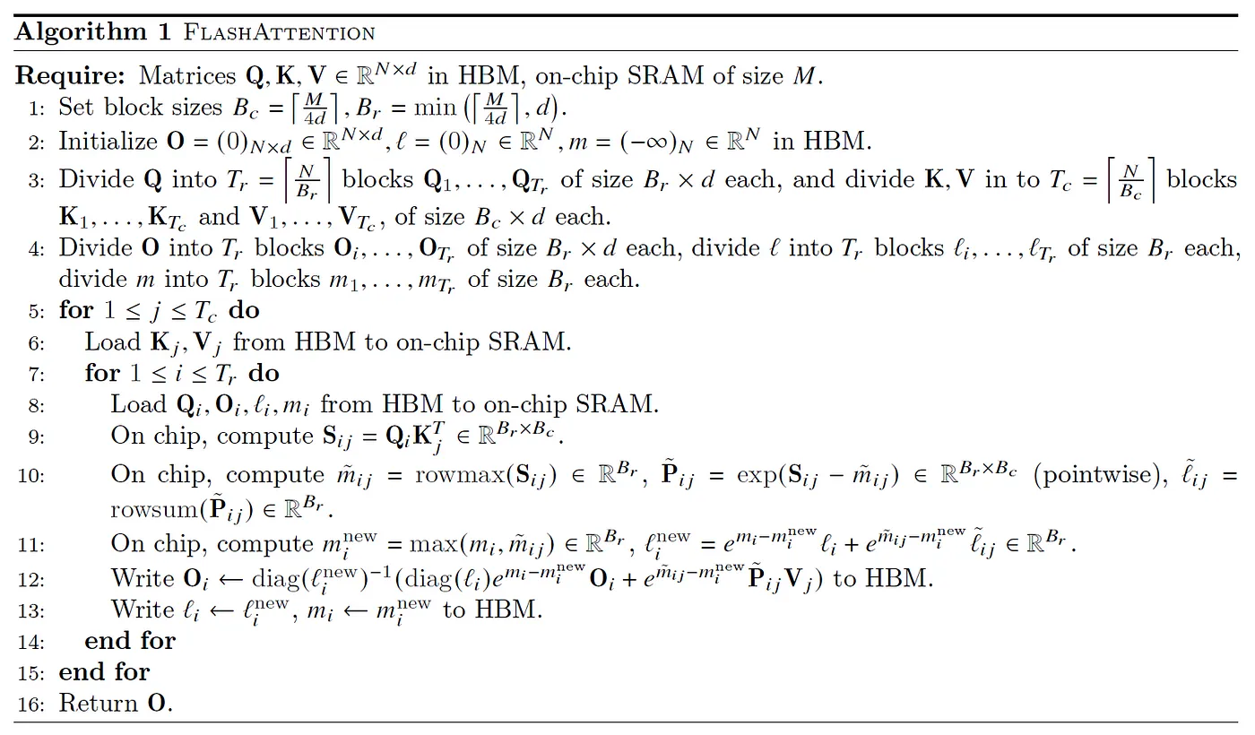
From a hardware standpoint, this lets us fit our chunk of Q into VMEM (what the algorithm above calls on-chip SRAM) so we only have to load the KV chunks on each iteration, increasing the arithmetic intensity. We can also keep the running statistics in VMEM.
从硬件的角度看,这让我们可以把 Q 的那一块塞进 VMEM(上面算法里叫 on-chip SRAM),于是每次迭代只需要加载 KV 块,从而提高了算术强度。我们还可以把 running 统计量也留在 VMEM 里。
One last subtle point worth emphasizing is an attention softmax property that’s used to make the Flash VJP (reverse mode derivative) calculation practical for training. We define an intermediate softmax array:
最后一个值得强调的微妙之处,是一个让 Flash 的 VJP(反向模式导数)计算在训练中变得可行的注意力 softmax 性质。我们定义一个中间 softmax 数组:
$$S_{ij} = \frac{e^{\tau q_i \cdot k_j}}{\sum_l e^{\tau q_i \cdot k_l}}$$
In attention, we obtain dS from reverse-mode dO and V arrays:
在注意力里,我们从反向模式的 dO 和 V 数组得到 dS:
$$dS_{ij} = dO_{id} \cdot_d V_{jd} = \sum_d dO_{id} V_{jd}$$
During the backpropagation of this gradient to Q and K
在把这个梯度反传到 Q 和 K 的过程中
$$d(q_i \cdot k_j) = (dS_{ij} - S_{ij} \cdot_j dS_{ij}) S_{ij}$$
We exploit an identity that allows us to exchange a contraction along the large key length dimension with a local contraction along the feature depth dimension.
我们利用一个恒等式,把沿很大的 key 长度维度的收缩,换成沿特征深度维度的局部收缩。
$$\begin{align*} S_{ij} \cdot_j dS_{ij} &= \sum_j \frac{e^{\tau q_i \cdot k_j}}{\sum_k e^{\tau q_i \cdot k_k}} \sum_d dO_{id} V_{jd} \\ &= \sum_d dO_{id} \sum_j \frac{e^{\tau q_i \cdot k_j}}{\sum_k e^{\tau q_i \cdot k_k}} V_{jd} \\ &= \sum_d dO_{id} O_{id} \\ &= dO_{id} \cdot_d O_{id} \end{align*}$$
This replacement is crucial for being able to implement a sequence-block local calculation for the VJP, and enables further clever sharding schemes like ring attention.
这个替换对于把 VJP 实现成序列块上的局部计算至关重要,也让 ring attention 之类更巧妙的方案成为可能。
讨论
用 GitHub 账号留言;评论保存在公开仓库chengshu-blog-discussions的 Discussions 里。也可通过 RSS 订阅后续文章。