如何扩展你的模型（1）：Roofline 分析入门

Where Does the Time Go?

Let’s start with an extremely simple question: why does an algorithm take 50ms instead of 50s or 5ms? What is actually happening within the model that takes substantial time and how long should we expect it to take?

Computation: A deep learning model is effectively a bunch of matrix multiplications, each composed of floating-point multiplication and addition ‘operations’ (FLOPs). Our accelerator speed determines how long these take to compute:

For instance, an NVIDIA H100 can perform about 9.89e14 bfloat16 (bf16 is short for bfloat16, a 16-bit floating point format often used in ML.) FLOPs/s while a TPU v6e can perform 9.1e14 FLOPs/s. (H100s and B200s can usually only achieve around 80-85% of the claimed peak FLOPs, while TPUs can get closer to 95% in normal use.) That means doing 1e12 FLOPs on an H100 will take (roughly) 1e12 / 9.89e14 = 1.01ms and 1e12 / 9.1e14 = 1.1ms on a TPU v6e. (Note that these chips are priced differently, and this comparison does not normalize to cost.)

Communication within a chip: Within an accelerator, tensors need to be transferred between accelerator memory (HBM) and the compute cores. You’ll see the bandwidth of this link referred to as “HBM bandwidth”. (NVIDIA also calls this “memory bandwidth.”) On an H100, this is about 3.35TB/s and on TPU v6e this is about 1.6TB/s.

Communication between chips: When we distribute a model across multiple accelerators, tensors frequently need to be transferred between them. There are often a few options for this on our hardware (ICI, DCN, and PCIe), each with different bandwidths.

Whether the communication is within a chip or between chips, we measure this in bytes/s and estimate the total communication time with:

Typically (but not always), computation within a single chip can be overlapped with communication within a chip and between chips. This means we can lower-bound training and inference time by using the maximum of computation and communication time. We can also upper-bound with their sum. In practice, we optimize against the maximum as the algebra is simpler and we can usually come close to this bound by overlapping our communication and computation. If we optimize with the maximum in mind then the lower and upper bounds differ by at most a factor of 2 since $T_\text{math} + T_\text{comms} \leq 2 * \max(T_\text{math}, T_\text{comms})$. We then increase accuracy beyond this by modeling ‘overlap regions’ and overheads, which can be informed by profiling your specific model and target system.

If we assume we can perfectly overlap communication and computation, when $T_\text{math} > T_\text{comms}$, we see full utilization from our hardware. We call this being “compute-bound”. When $T_\text{comms} > T_\text{math}$, we tend to be “communication-bound” (We’ll use “communication-bound”, “comms-bound”, “memory-bound”, and “bandwidth-bound” interchangeably throughout this book.) and at least some fraction of our accelerator FLOPs/s is wasted waiting for data to be passed around. One way to tell if an operation will be compute or communication-bound is to look at its “arithmetic intensity” or “operational intensity”.

Definition: the arithmetic intensity of an algorithm is given by the ratio of the total FLOPs it performs to the number of bytes it needs to communicate — either within a chip or between chips.

Arithmetic intensity measures the “FLOPs per byte” of a given operation. To a first order, when our arithmetic intensity is high, $T_\text{math}$ is large compared to $T_\text{comms}$ and we typically use most of the available FLOPs. When the opposite is true, we spend more time on comms and waste FLOPs. The point where this crossover happens is the “peak arithmetic intensity” of our hardware, the ratio of peak accelerator FLOPs/s to accelerator bandwidth.

The quantity $\text{Intensity}(\text{Accelerator})$ is the arithmetic intensity at which our accelerator achieves its peak FLOPs/s. For the TPU v5e MXU, this is about 240 FLOPs/byte, since the TPU can perform 1.97e14 FLOPs/s and load 8.2e11 bytes/s from HBM. (The MXU is the matrix multiply unit on the TPU. We specify this here because the TPU has other accelerators like the VPU that are responsible for elementwise operations that have a different peak FLOPs/s.) That means if an algorithm has a lower arithmetic intensity than 240 FLOPs/byte, it will be bound by byte loading and thus we won’t make good use of our hardware. (This is only true if the algorithm loads its weights from HBM and runs in the MXU. As we’ll discuss in the next section, we can sometimes store parameters in VMEM which has a much higher bandwidth. Many algorithms also run in the VPU, which has different performance characteristics.) Let’s look at one such example:

Example (dot product): to compute the dot product of two vectors in bfloat16 precision, x • y: bf16[N], bf16[N] → bf16[1], we need to load $x$ and $y$ from memory, each of which has $2 * N = 2N$ bytes, perform $N$ multiplications and $N-1$ additions, and write $2$ bytes back into HBM $$\begin{equation} \text{Intensity}(\text{dot product}) = \frac{\text{Total FLOPs}}{\text{Total Bytes}} = \frac{N + N - 1}{2N + 2N + 2} = \frac{2N - 1}{4N + 2} \rightarrow \frac{1}{2} \end{equation}$$

as $N\rightarrow\infty$. So the dot product has an arithmetic intensity of $\frac{1}{2}$ or, put another way, the dot product does 0.5 floating point operations per byte loaded. This means our arithmetic intensity is lower than that of our hardware and we will be communication-bound. (The 240 number above is not the correct comparison here since, as you will see in the next section, a dot-product is performed on the VPU and not the MXU. The TPU v5p VPU can do roughly 7e12 FLOPs / second per core, so its critical intensity is around 3, which means we are still somewhat comms-bound here. Either way, the fact that our intensity is low and constant means it is difficult to be compute-bound on most hardware.)

Visualizing rooflines

We can visualize the tradeoff between memory and compute using a roofline plot, which plots the peak achievable FLOPs/s (throughput) of an algorithm on our hardware (the y-axis) against the arithmetic intensity of that algorithm (the x-axis). Here’s an example log-log plot:

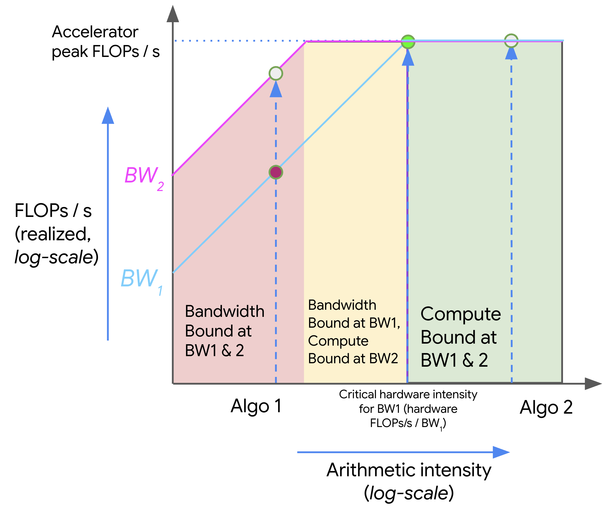
Above, as the intensity increases (moving left to right), we initially see a linear increase in the performance of our algorithm (in FLOPs/s) until we hit the critical arithmetic intensity of the hardware, 240 in the case of the TPU v5e. Any algorithm with a lower intensity will be bandwidth (BW) bound and limited by the peak memory bandwidth (shown in red). Any algorithm to the right will fully utilize our FLOPs (shown in green). Here, Algo 1 is comms-bound and uses only a fraction of the total hardware FLOPs/s. Algo 2 is compute-bound. We can generally improve the performance of an algorithm either by increasing its arithmetic intensity or by increasing the memory bandwidth available (moving from BW1 to BW2).

Matrix multiplication

Let’s look at our soon-to-be favorite algorithm: matrix multiplication (aka matmul). Given two matrices $X$ and $Y$, we can write $X * Y \rightarrow Z$ where $X$ has shape $\text{bf16}[B, D]$, $Y$ has shape $\text{bf16}[D, F]$, and $Z$ has shape $\text{bf16}[B, F]$. To do the matmul we need to load $2DF + 2BD$ bytes, perform $2BDF$ FLOPs, and write $2BF$ bytes back. (Technically we perform $BF \times (2D - 1)$ FLOPs but this is close enough. This comes from $BDF$ multiplications and $BF * (D-1)$ additions. Section 4 has more details.) (Although the output of a matmul is technically float32 we usually cast down to bfloat16 before copying back to HBM.) Thus:

We can get a nice simplification if we assume our “batch size” $B$ is small relative to $D$ and $F$. Then we get

This is a reasonable assumption for Transformer matmuls since we typically have a local (per-replica) token batch size $B < 1024$ (note, not sequences) but $D$ and $F > 8000$. Thus we generally become compute-bound when our per-replica (We say per-replica because, if we do some kind of model sharding to increase the number of chips used in the matmul, we scale both our available compute and memory bandwidth by the same amount. Thus the critical batch size is true per independent copy of the model weights.) batch size is greater than 240 tokens, a very simple rule!

Takeaway: for a bfloat16 matmul to be compute-bound on most TPUs, we need our batch size to be greater than 240 (tokens). (Note that this is not the batch size in the usual sense, where it means the batch size in sequences. It turns out most rooflines depend purely on the number of tokens, whether they belong to the same or different sequences. For instance if you have a batch size of 512 sequences of 4096 tokens on 2048 GPUs, you have a total batch size of 512 * 4096 = 2M tokens, and a local batch size of 1k tokens.)

This comes with a few notable caveats we’ll explore in the problems below, particularly with respect to quantization (e.g., if we quantize our activations but still do full-precision FLOPs), but it’s a good rule to remember. For GPUs, this number is slightly higher (closer to 300), but the same conclusion generally holds. When we decompose a big matmul into smaller matmuls, the tile sizes also matter. (When we do a large matrix multiplication, we need to break it down into smaller tiles which fit into VMEM/SMEM/TMEM, the higher-bandwidth on-chip memory. This causes us to load chunks multiple times, so it’s no longer quite true that we only load $O(N^2)$ bytes. Consider an $(m, k) \cdot (k, n)$ matmul with tile sizes $bm$, $bk$, $bn$. Let $tm = m / bm$, etc. Then the total FLOPs is $2 \cdot tm \cdot tn \cdot tk \cdot bm \cdot bn \cdot bk$ and the total bytes are $2 \cdot tm \cdot tn \cdot (tk \cdot (bm \cdot bk + bk \cdot bn) + bm \cdot bn)$. Ignoring the last term, we have an intensity of $bm \cdot bn / (bm + bn)$, which is similar to the above.) We’ll discuss the lower-level GPU and TPU details in the next section.

Network communication rooflines

All the rooflines we’ve discussed so far have been memory-bandwidth rooflines, all within a single chip. This shouldn’t be taken as a rule. In fact, most of the rooflines we’ll care about in this book involve communication between chips: usually matrix multiplications that involve matrices sharded across multiple TPUs.

To pick a somewhat contrived example, say we want to multiply two big matrices $X\sim \text{bf16}[B, D]$ and $Y \sim \text{bf16}[D, F]$ which are split evenly across 2 TPUs/GPUs (along the $D$ dimension). To do this multiplication (as we’ll see in Section 3), we can multiply half of each matrix on each TPU (Z0 = X[:, :D // 2] @ Y[:D // 2, :] on TPU 0 and Z1 = X[:, D // 2:] @ Y[D // 2:, :] on TPU 1) and then copy the resulting “partial sums” to the other TPU and add them together. Say we can copy 4.5e10 bytes/s in each direction and perform 1.97e14 FLOPs/s on each chip. What are $T_\text{math}$ and $T_\text{comms}$?

$T_\text{math}$ is clearly half of what it was before, since each TPU is doing half the work, i.e. (We’re ignoring the FLOPs required to add the two partial sums together (another BF addition), but this is basically negligible.)

Now what about $T_\text{comms}$? This now refers to the communication time between chips! This is just the total bytes sent divided by the network bandwidth, i.e.

Therefore we become compute-bound (now with respect to the inter-chip network) when $$\text{Intensity}(\text{matmul (2-chips)}) > \text{Intensity}(\text{TPU w.r.t. inter-chip network})$$ or equivalently when $\frac{BDF}{2BF} = \frac{D}{2} > \frac{1.97e14}{4.5e10} = 4377$ or $D > 8755$. Note that, unlike before, the critical threshold now depends on $D$ and not $B$! Try to think why that is. This is just one such example, but we highlight that this kind of roofline is critical to knowing when we can parallelize an operation across multiple TPUs.

A Few Problems to Work

Question 1 [int8 matmul]: Say we want to do the matmul $X[B, D] \cdot_D Y[D, F] \rightarrow Z[B, F]$ (Here and throughout we’ll use the notation $A \cdot_D B$ to indicate that the multiplication is performing a contraction over the D dimension. This is an abuse of einsum notation.) in int8 precision (1 byte per parameter) instead of bfloat16 (2 bytes per parameter) since TPUs/GPUs can do matmuls faster in lower precision.

1. How many bytes need to be loaded from memory? How many need to be written back to memory?
2. How many total OPs are performed?
3. What is the arithmetic intensity?
4. What is a roofline estimate for $T_\text{math}$ and $T_\text{comms}$? What are reasonable upper and lower bounds for the runtime of the whole operation?

Assume our HBM bandwidth is 8.2e11 bytes/s and our int8 peak OPs/s is 3.94e14 (about 2x bfloat16).

1. Because we’re storing our parameters in int8, we have 1 byte per parameter, so we have $$BD + DF$$ bytes loaded from HBM and $$BF$$ written back.
2. This is the same as in bfloat16, but in theory int8 OPs/s should be faster. So this is still $2BDF$ OPs.
3. Arithmetic intensity is $$2BDF / (BD + DF + BF)$$. If we make the same assumption as above about $$B \ll D$$ and $$B \ll F$$, we get an arithmetic intensity of $$2B$$, meaning our rule becomes $B > \text{HBM int8 arithmetic intensity} / 2$. Using the numbers given, this int8 intensity is 3.94e14 / 8.2e11 = 480, so the rule is $B > 480 / 2 = 240$. Note that this is basically unchanged!
4. $$T_\text{math} = 2BDF / 3.94e14$$ and $$T_\text{comms} = (BD + DF + BF) / 8.2e11$$, so a reasonable lower bound is $$\max(T_\text{math}, T_\text{comms})$$ and an upper bound is $$T_\text{math} + T_\text{comms}$$.

Question 2 [int8 + bf16 matmul]: In practice we often do different weight vs. activation quantization, so we might store our weights in very low precision but keep activations (and compute) in a higher precision. Say we want to quantize our weights in int8 but keep activations (and compute) in bfloat16. At what batch size do we become compute bound? Assume 1.97e14 bfloat16 FLOPs/s.

Hint: this means specifically bf16[B, D] * int8[D, F] -> bf16[B, F] where $B$ is the “batch size”.

Again assuming B is small, we have 2BDF bfloat16 FLOPs but only DF weights (instead of 2DF in bfloat16). This means we become compute-bound when $$2B > 240$$ or $$B > 120$$. This is a lot lower, meaning if we can do int8 weight quantization (which is fairly easy to do) but still do bfloat16 FLOPs, we get a meaningful win in efficiency (although int8 OPs would be better).

Question 3: Taking the setup from Question 2, make a roofline plot of peak FLOPs/s vs. $B$ for $F = D = 4096$ and $F = D = 1024$. Use the exact number of bytes loaded, not an approximation.

Here is the plot in question:

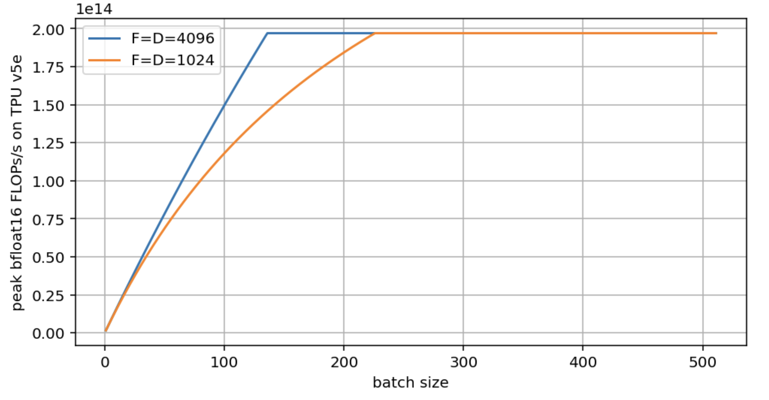
Note that both models eventually achieve the peak hardware FLOPs/s, but the larger D/F achieve it sooner. D=F=1024 almost doubles the critical batch size. The code to generate this figure is here:

Question 4: What if we wanted to perform $\text{int8}[B, D] \cdot_D \text{int8}[B, D, F] \rightarrow \text{int8}[B, F]$ where we imagine having a different matrix for each batch element. What is the arithmetic intensity of this operation?

Let’s start by looking at the total FLOPs and comms.

1. Total FLOPs: the FLOPs is basically the same, since we’re doing $$B$$ independent $$[D] \times [D, F]$$ products, the same total work as a single $$[B, D] \times [D, F]$$ matmul (this is discussed more in Section 4). So this is just $$2BDF$$.
2. Total comms: we have a lot more comms here: $$BD + BDF + BF$$.
3. Therefore, our arithmetic intensity is now actually $$2BDF / (BD + BDF + BF)$$. Since $$BDF$$ dominates the denominator, this is roughly $$2$$. So instead of it depending on the batch size, this is essentially constant. This is bad because it means we’ll basically always be comms bound no matter what.

Question 5 [Memory Rooflines for GPUs]: Using the spec sheet provided by NVIDIA for the H100 SXM, calculate the batch size at which a bfloat16 matrix multiplication will become compute-bound. Note that the Tensor Core FLOPs numbers are twice the true value since they’re only achievable with structured sparsity.

From the spec sheet, we see that the reported bfloat16 FLOPs value is 1.979e15 FLOPs/s with an asterisk noting “with sparsity”. The true value is half this without sparsity, i.e. 9.89e14 FLOPs/s. The memory bandwidth is 3.35TB/s, or 3.35e12 bytes / second. Thus $B_\text{crit}$ is 9.89e14 / 3.35e12 = 295, rather similar to the TPU.

That’s it for Part 1! For Part 2, looking at how real TPUs handle FLOPs and communication, click here.