《让深度学习跑出 Brrrr》中英对照全译:从第一性原理看清 compute、带宽与 overhead
Horace He 的经典长文《Making Deep Learning Go Brrrr From First Principles》全文对照翻译:左栏英文原文、右栏中文译文。用「工厂」类比讲清 compute / memory bandwidth / overhead 三种性能 regime,以及 operator fusion、compute intensity、CUDA Graph 这些优化的适用边界。
原文:Making Deep Learning Go Brrrr From First Principles,作者 Horace He,2022 年。
本站是中英对照排版:左栏是英文原文,右栏是对应的中文译文。不好翻译的术语(compute、memory bandwidth、overhead、operator fusion、compute intensity、regime 等)保留英文写法;原文配图全部保留,并标注出处。
So, you want to improve the performance of your deep learning model. How might you approach such a task? Often, folk fall back to a grab-bag of tricks that might’ve worked before or saw on a tweet. “Use in-place operations! Set gradients to None! Install PyTorch 1.10.0 but not 1.10.1!”
所以,你想提升自己深度学习模型的性能。你会怎么下手?很多时候,大家会翻出一堆杂七杂八的招数——以前碰巧管用过的,或者在推特上刷到过的。“用 in-place 操作!把梯度设成 None!装 PyTorch 1.10.0,但千万别装 1.10.1!”
It’s understandable why users often take such an ad-hoc approach performance on modern systems (particularly deep learning) often feels as much like alchemy as it does science. That being said, reasoning from first principles can still eliminate broad swathes of approaches, thus making the problem much more approachable.
用户为什么经常用这种临时凑合的方式调性能,其实不难理解:在现代系统上,尤其是深度学习,性能这件事给人的感觉更像是炼金术,而不是科学。话虽如此,从第一性原理出发进行推理,依然可以直接排除掉一大片做法,让问题变得好下手得多。
For example, getting good performance on a dataset with deep learning also involves a lot of guesswork. But, if your training loss is way lower than your test loss, you’re in the “overfitting” regime, and you’re wasting your time if you try to increase the capacity of your model. Or, if your training loss is identical to your validation loss, you’re wasting your time if you try to regularize your model.
举个例子:用深度学习在某个数据集上跑出好成绩,同样要靠大量猜测。但如果你发现训练 loss 远低于测试 loss,那你正处在“过拟合”这个 regime 里,这时再去加大模型容量就是浪费时间。反过来,如果训练 loss 和验证 loss 一模一样,那你再去给模型加正则化也是白费功夫。
Similarly, you can understand efficiency of your deep learning regime as consisting of 3 different components.
同样的道理,你可以把深度学习系统的效率拆成三个组成部分。
- Compute: Time spent on your GPU computing actual floating point operations (FLOPS)
- Memory: Time spent transferring tensors within a GPU
- Overhead: Everything else
- Compute:GPU 花在真正做浮点运算(FLOPS)上的时间
- Memory:在 GPU 内部搬运 tensor 所花的时间
- Overhead:其他所有东西
Just like with training ML models, knowing what regime you’re in allows you to narrow in on optimizations that matters. For example, if you’re spending all of your time doing memory transfers (i.e. you are in an memory-bandwidth bound regime), then increasing the FLOPS of your GPU won’t help. On the other hand, if you’re spending all of your time performing big chonky matmuls (i.e. a compute-bound regime), then rewriting your model logic into C++ to reduce overhead won’t help.
就像训练 ML 模型时一样,知道自己身处哪个 regime,就能把精力收拢到真正重要的优化上。比如,如果你的时间全花在搬运数据上(也就是处在 memory-bandwidth bound regime),那么去提升 GPU 的 FLOPS 根本没用。反过来,如果你的时间全花在做又大又粗的 matmul 上(也就是 compute-bound regime),那把模型逻辑用 C++ 重写来降低 overhead 也没用。
So, if you want to keep your GPUs going brrrr, let’s discuss the three components your system might be spending time on - compute, memory bandwidth, and overhead.
所以,想让你的 GPU 一直 brrrr 下去,我们就来聊聊系统可能把时间花掉的三样东西——compute、memory bandwidth 和 overhead。
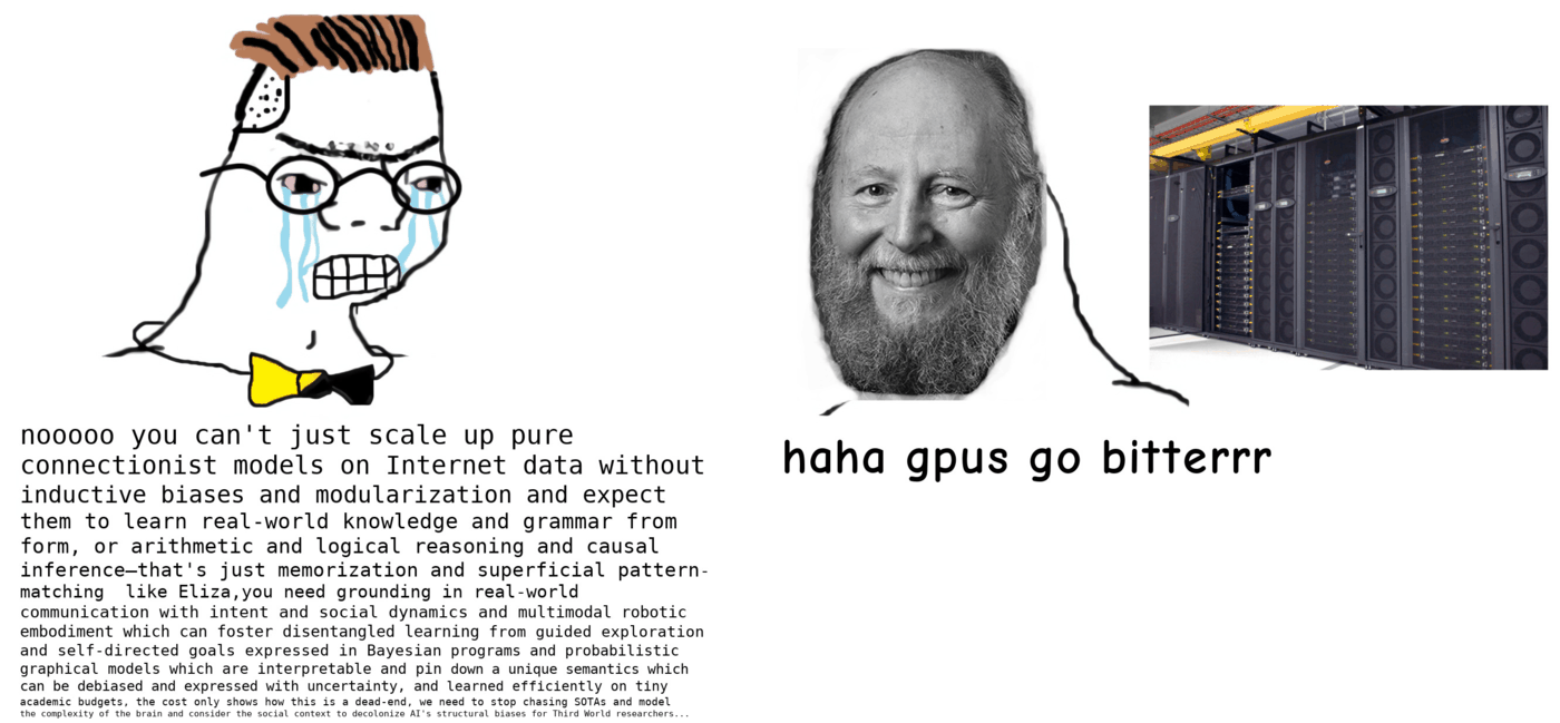
Note: Most of this post will use GPUs and PyTorch as examples (as I work on the PyTorch team), but the principles almost all generalize across hardware and frameworks.
注:本文大部分例子会以 GPU 和 PyTorch 为主(因为我在 PyTorch 团队工作),但这些原理几乎都能推广到别的硬件和框架。
Compute
计算
One perspective on optimizing deep learning systems is that we’d like to maximize the time in the compute-bound regime. You paid for all of those 312 teraflops, and ideally, you’d get those 312 teraflops. But, in order to get your money’s worth out of your expensive matrix multiplication, you need to reduce the amount of time spent in the other parts.
优化深度学习系统的一种视角是:我们想把处在 compute-bound regime 的时间尽量拉满。那 312 teraflops 是你花了钱买来的,理想情况下你就该实实在在地拿到这 312 teraflops。但要想让你那些昂贵的矩阵乘法物有所值,你就得减少花在其他部分上的时间。
But why the focus on maximizing compute and not say, memory bandwidth? The reason is simple - you can reduce the overhead or memory costs, but you (mostly) can’t reduce the computation required without changing the actual operations you’re performing.
那为什么盯着“最大化 compute”,而不是比如 memory bandwidth?理由很简单:overhead 和访存成本都是可以压缩的,但如果不改变你实际要做的运算,你(基本上)没法减少所需的计算量。
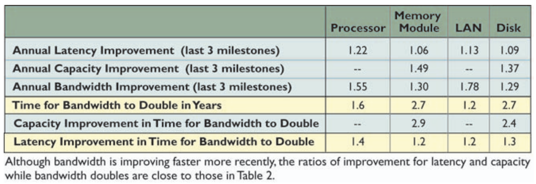
Exacerbating the difficulty of maximizing compute utilization is the rate at which compute grows compared to memory bandwidth. Take this table on CPU FLOPS doubling times vs. memory bandwidth doubling times
更麻烦的是,compute 的增长速度和 memory bandwidth 根本不在一个量级。看看这张表,它列出了 CPU 的 FLOPS 翻倍所需时间与 memory bandwidth 翻倍所需时间的对比。
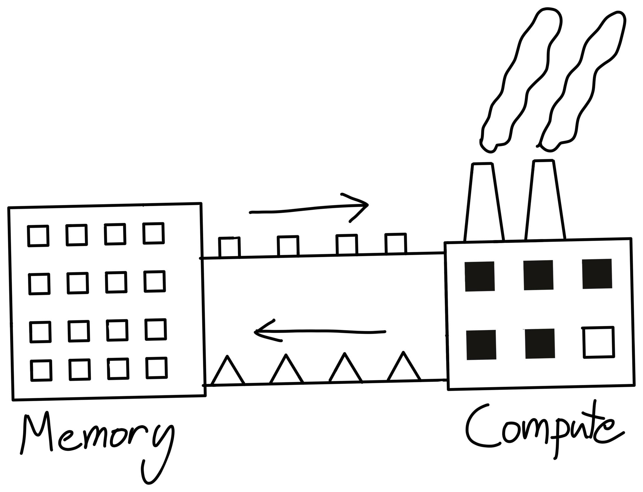
One way to think about compute is as a factory. We send instructions to our factory (overhead), send it materials (memory-bandwidth), all to keep our factory running efficiently (compute).
可以把 compute 想象成一座工厂。我们给工厂下指令(overhead),给工厂送原料(memory bandwidth),目的都是让这座工厂高效地运转(compute)。
So, if our factory increases efficiency faster than the rate at which we can supply it materials, it becomes harder for our factory to achieve its peak efficiency.
于是,如果工厂提升效率的速度快过我们给它送原料的速度,这座工厂就越难达到它的峰值效率。
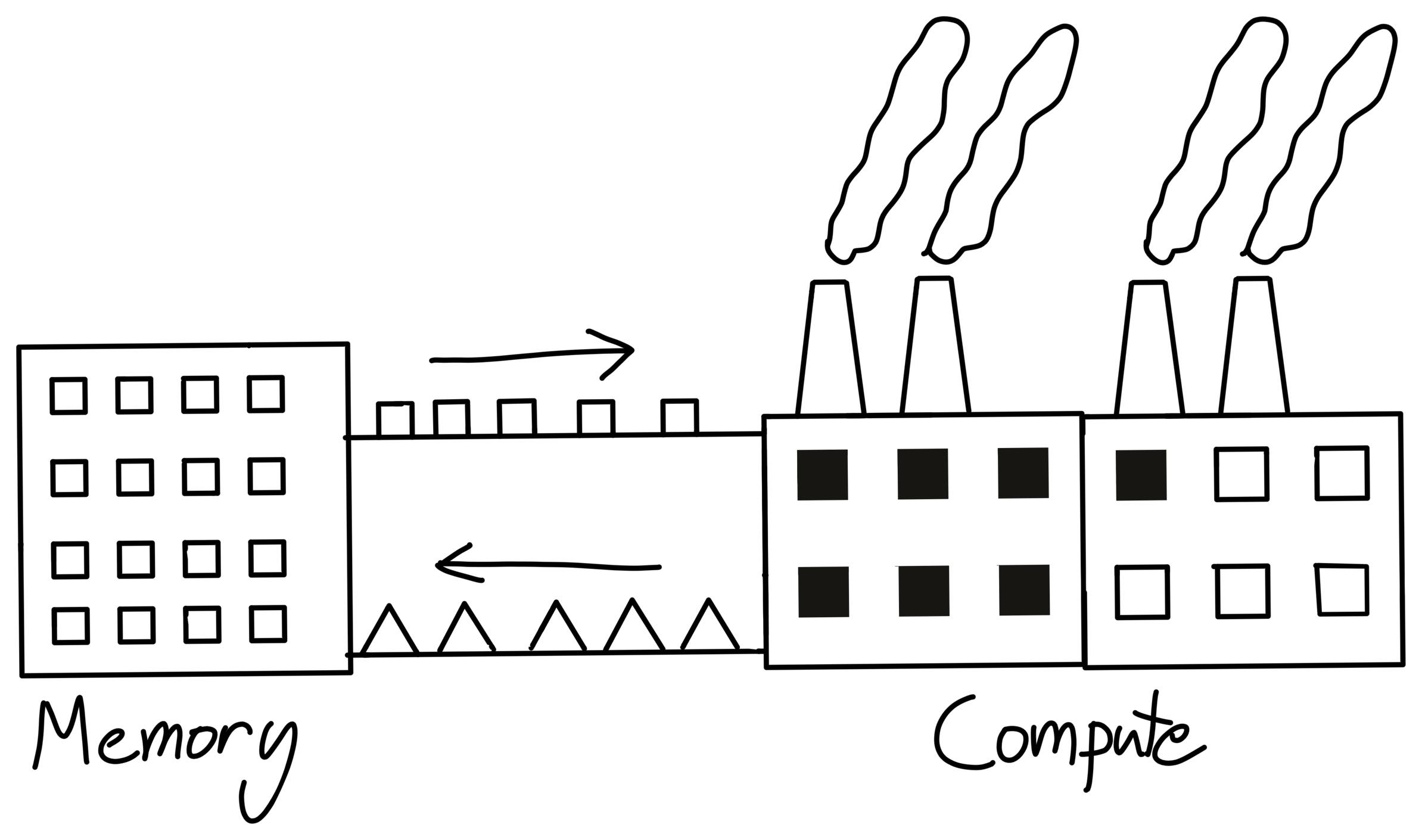
Even though our factory's size (FLOPS) doubled - if our bandwidth can't keep up then our performance isn't also going to double
Along with implying permanent job security for ML systems engineers, this growing difficulty in utilizing our compute also makes understanding our bottlenecks even more important.
这种“算力越来越难用满”的趋势,一方面意味着 ML 系统工程师永远不会失业,另一方面也让我们更有必要搞清楚自己的瓶颈到底在哪。
One more addendum about FLOPS. Modern machine learning accelerators all have hardware specialized for matrix-multiplication, such as Nvidia’s “Tensor Cores”.
关于 FLOPS 再补一句。现代机器学习加速器都有专门为矩阵乘法设计的硬件,比如 Nvidia 的 “Tensor Cores”。
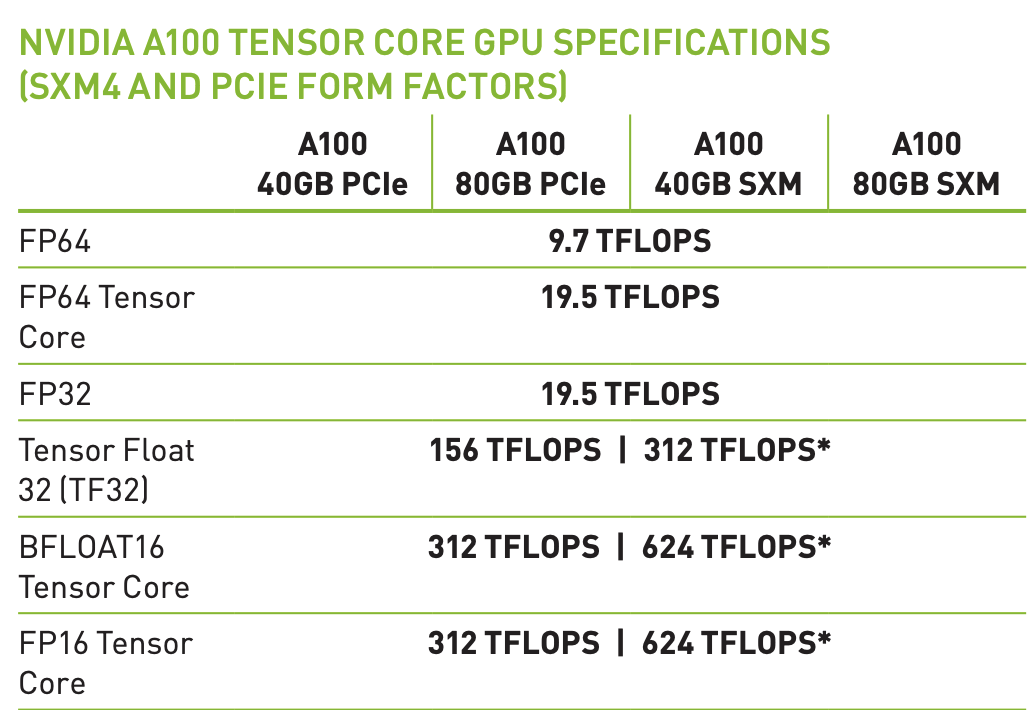
So, if you aren’t doing matrix multiplication, you’ll only be able to achieve 19.5 teraflops instead of the stated 312. Note that this isn’t unique to GPUs - in fact, TPUs are even less general than GPUs.
所以,如果你不做矩阵乘法,实际能拿到的就只有 19.5 teraflops,而不是标称的 312。注意这不是 GPU 独有的问题——事实上,TPU 的通用性比 GPU 还要差。
The fact that GPUs are so much slower at everything that isn’t a matrix multiply might seem problematic at first - what about our other operators like layer norm or activation functions? Well, the truth is, those operators are just rounding errors in terms of FLOPS. For example, let’s look at this table of FLOP counts on BERT for different operator types from this paper, where “Tensor Contraction” = matmuls.
GPU 在所有非矩阵乘法的操作上都慢得多,这一点乍看像是大问题——那 layer norm、激活函数这些算子怎么办?其实真相是:这些算子在 FLOPS 总量里只是舍入误差级别的存在。举个例子,看看这篇论文里 BERT 上不同算子类型的 FLOP 数表格,其中 “Tensor Contraction” 指的就是 matmul。
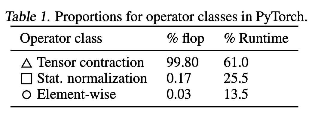
You can see that altogether, our non-matmul ops only make up 0.2% of our FLOPS, so it doesn’t matter that our GPU computes non-matmul ops 15x slower.
可以看到,非 matmul 算子加起来只占全部 FLOPS 的 0.2%,所以 GPU 算这些算子慢 15 倍也无所谓。
But, in this case, the normalization and pointwise ops actually achieve 250x less FLOPS and 700x less FLOPS than our matmuls respectively.
但在这个例子里,normalization 和 pointwise 算子实际达到的 FLOPS,分别比 matmul 少了 250 倍和 700 倍。
So why do our non-matmul ops take so much more time than they should?
那为什么非 matmul 算子花的时间比“应有的”多这么多?
Going back to our analogy, the culprit is often how long it takes to transport materials to and from the factory. In other words, the memory bandwidth.
回到那个类比:罪魁祸首往往是原料运进运出工厂的时间。换句话说,就是 memory bandwidth。
Bandwidth
带宽
Bandwidth costs are essentially the cost paid to move data from one place to another. This might be moving the data from CPU to GPU, from one node to another, or even from CUDA global memory to CUDA shared memory. This last one, in particular, is what we’ll be focusing on here, and is typically referred to as “bandwidth cost” or “memory bandwidth cost”.
带宽成本,本质上就是把数据从一个地方搬到另一个地方所付出的代价。这可能是把数据从 CPU 搬到 GPU,从一个节点搬到另一个节点,甚至是从 CUDA global memory 搬到 CUDA shared memory。这里我们重点讲最后一种,它通常就被称为 “bandwidth cost” 或 “memory bandwidth cost”。
The other two (typically referred to as “data transfer costs” and “network costs” respectively) are certainly important, but going into distributed performance would cause me to never finish this post.
另外两种(通常分别叫 “data transfer costs” 和 “network costs”)当然也很重要,但一旦扯进分布式性能,这篇文章我就永远写不完了。
To understand what the memory bandwidth cost is, let’s head back to our factory analogy.
要理解什么是 memory bandwidth 成本,我们再回到工厂那个类比。
Although our factory is where we do the actual work, it’s not suitable as a bulk storage unit. A large part of this is that since we’re doing actual work here, all the storage is optimized for being fast to actually use (SRAM), instead of having a lot of it.
工厂是我们实际干活的地方,但它不适合当大宗仓库。很大程度上是因为:既然这里要干活,那么所有存储都是为了让数据用起来快(SRAM)而优化的,而不是为了让它多。
So, where do we store the actual results and materials? The typical approach is to have a warehouse, probably somewhere where land is cheap and we have a lot of space (DRAM). Then, we can ship supplies to and from our factories (memory bandwidth).
那真正的成品和原料存哪儿?通常的做法是搞一个仓库,多半选在地价便宜、空间充足的地方(DRAM)。然后我们就能在工厂和仓库之间来回运货(memory bandwidth)。
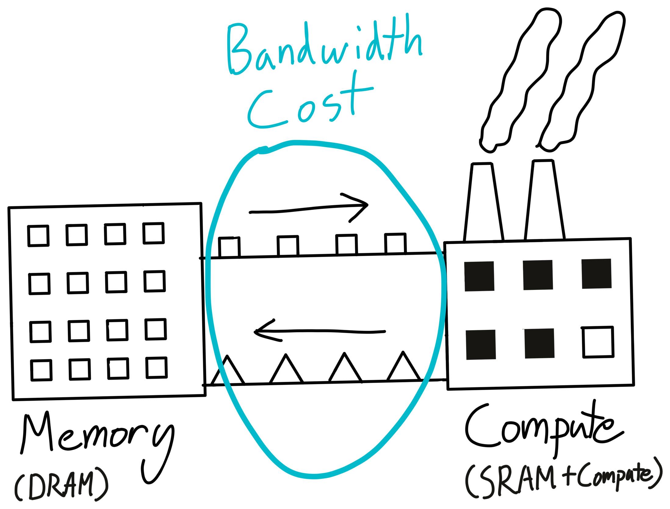
This cost of moving stuff to and from our compute units is what’s called the “memory bandwidth” cost. As an aside, your GPU’s DRAM is what shows up in nvidia-smi, and is the primary quantity responsible for your lovely “CUDA Out of Memory’ errors.
这种在计算单元之间来回搬运东西的成本,就叫 “memory bandwidth” 成本。顺带一提,nvidia-smi 里显示的就是 GPU 的 DRAM 用量,它也是你那些可爱的 “CUDA Out of Memory” 报错的主要元凶。
One thing to note is that every single time we perform a GPU kernel, we need to move our data from and back to our GPU’s DRAM (i.e. our warehouse).
需要注意的一点是:每执行一次 GPU kernel,我们都要把数据从 GPU 的 DRAM(也就是仓库)里搬出来,再搬回去。
Now, imagine what happens when we perform an unary operation like torch.cos. We need to ship our data from our storage to the warehouse, then perform a tiny bit of computation for each piece of data, and then ship that storage back. Shipping things around is quite expensive. As a result, nearly all of our time here is spent shipping data around, and not on the actual computation itself.
现在想象一下执行一个一元操作(比如 torch.cos)会发生什么。我们要把数据从仓库运到计算单元,对每个元素做一点点计算,然后再把结果运回仓库。搬运本身相当贵,结果是这里几乎所有时间都花在搬运上,而不是花在真正的计算上。
Since we’re spending all of our time on memory-bandwidth, such an operation is called a memory-bound operation, and it means that we’re not spending a lot of time on compute.
由于时间几乎全花在 memory bandwidth 上,这类操作被称为 memory-bound operation,意思是我们在 compute 上并没有花多少时间。
Ok, so that’s not ideal. What can we do about it? Let’s take a look at how a sequence of operators might look.
好吧,这并不理想。能怎么办呢?我们来看看一串算子连起来执行时是什么样子。
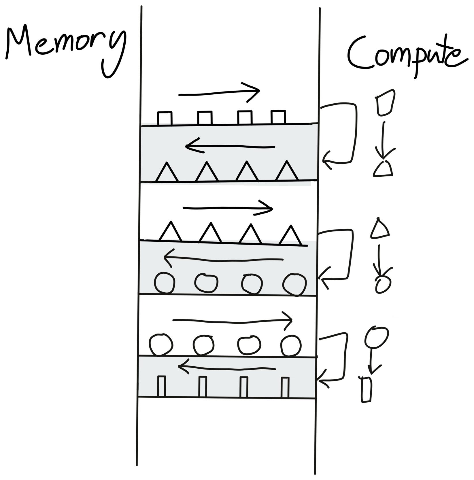
Here's how a sequence of pointwise operators might look like.
Hey! This is a very stupid arrangement. Why are we sending the same data to global memory and then back to the compute units, over and over? We should just keep the data at the factory, perform all of our compute, and then send it back!
嘿!这个安排蠢透了。为什么要把同一份数据一遍遍地送去 global memory 再搬回计算单元?我们大可以把数据留在工厂里,把所有计算都做完,然后再送回去!
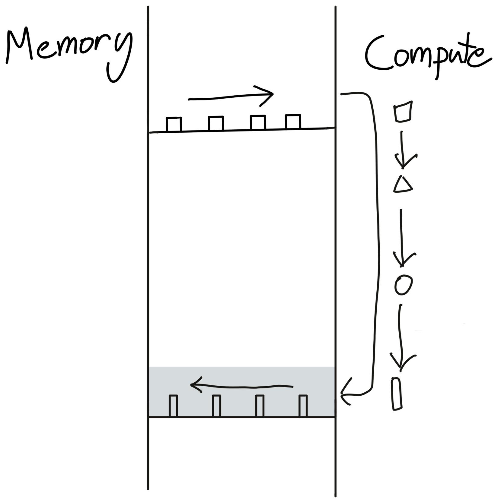
Instead of sending our triangle back to global memory just to read it back again, we instead just do all of our operations in one go.
This is operator fusion - the most important optimization in deep learning compilers. Simply put, instead of writing our data to global memory just to read it again, we elide the extra memory accesses by performing several computations at once.
这就是 operator fusion(算子融合)——深度学习编译器里最重要的优化。简单说,与其把数据写进 global memory 只为再读一次,我们干脆一次做完好几个计算,把多余的访存省掉。
For example, if we perform x.cos().cos(), usually we need to perform 4 global reads and writes.
举个例子,执行 x.cos().cos() 时,通常需要 4 次 global memory 读写。
x1 = x.cos() # Read from x in global memory, write to x1
x2 = x1.cos() # Read from x1 in global memory, write to x2
But, with operator fusion, we only need 2 global memory reads and writes! So operator fusion will speed it up by 2x.
但有了 operator fusion,只需要 2 次 global memory 读写!于是 operator fusion 把它加速了 2 倍。
x2 = x.cos().cos() # Read from x in global memory, write to x2Much better.
好多了。
There are a couple of caveats that make this a bit tricky. First of all, the GPU needs to know what’s going to happen next when performing the current operation. So, you can’t do this optimization in eager-mode, where PyTorch runs operators one at a time. Second, we actually need to generate CUDA code for this, which opens up a whole new can of worms.
有几个坑让这件事变得有点麻烦。首先,GPU 在执行当前算子时,需要知道下一步要做什么。所以这个优化没法在 eager 模式下做——eager 模式下 PyTorch 是一个算子一个算子地执行的。其次,我们实际上需要为此生成 CUDA 代码,这又打开了一个全新的麻烦盒子。
Not all operator fusion is as simple as pointwise operators. You can fuse pointwise operators onto reductions, or pointwise operators onto matrix multiplication. Even matrix multiplication itself can be thought of as fusing a broadcasting multiply followed by a reduction.
并不是所有 operator fusion 都像 pointwise 算子那么简单。你可以把 pointwise 算子融合到 reduction 上,也可以把它融合到矩阵乘法上。甚至矩阵乘法本身,都可以看成是“先做一次广播乘法、再做一次 reduction”的融合。
If you’re interested in writing custom CUDA kernels, it’s likely that this is where you’ll see the most benefit. Any 2 PyTorch operators present an opportunity for fusion, thus saving the memory bandwidth costs of reading/writing out to global memory between them. In addition, many existing compilers can often perform “simple” fusions - NVFuser and XLA being two examples. However, automated systems are no match for human ingenuity, so if you want to try out writing some custom CUDA kernels yourself, Triton is a great place to start.
如果你想自己写自定义 CUDA kernel,这大概是最能看到收益的地方。任意两个 PyTorch 算子之间都存在融合的机会,能省掉它们在 global memory 之间来回读写的 memory bandwidth 成本。此外,很多现有编译器已经能完成“简单”的融合——NVFuser 和 XLA 就是两个例子。不过自动化系统终究比不过人的巧思,所以如果你想自己动手写点自定义 CUDA kernel,Triton 是个很好的起点。
Finally, operator fusion leads to some surprising consequences. For one, a fused x.cos().cos() will take nearly the exact same time as calling x.cos() by itself. This is why activation functions are nearly all the same cost, despite gelu obviously consisting of many more operations than relu.
最后,operator fusion 还会带来一些反直觉的结果。其中之一:融合后的 x.cos().cos() 耗时几乎和单独调用一次 x.cos() 完全一样。这就是为什么各种激活函数的开销几乎都差不多——尽管 gelu 显然比 relu 包含多得多的运算。
This fact leads to some interesting consequences for rematerialization/activation checkpointing. Essentially, doing extra recomputation might lead to less memory-bandwidth, and thus less runtime. Thus, we can lower both memory and runtime through rematerialization, which we leveraged to build a neat min-cut optimization pass in AOTAutograd. You can read more about it here (might also go into it in a future blog post!)
这个事实对 rematerialization / activation checkpointing 有一些很有意思的推论。本质上,多做一次重算反而可能带来更少的 memory bandwidth 消耗,从而缩短运行时间。也就是说,通过 rematerialization,我们可以同时降低 memory 和运行时间——我们正是利用这一点,在 AOTAutograd 里做了一个漂亮的 min-cut 优化 pass。想深入了解可以看这里(以后也可能单独写一篇博客来讲!)
Reasoning about Memory-Bandwidth Costs
关于显存带宽成本的推理
When it come to reasoning about whether your operation is memory-bandwidth bound, a calculator can go a long way.
要判断一个操作是不是 memory-bandwidth bound,一个计算器就能帮你走很远。
For simple operators, it’s feasible to reason about your memory bandwidth directly. For example, an A100 has 1.5 terabytes/second of global memory bandwidth, and can perform 19.5 teraflops/second of compute. So, if you’re using 32 bit floats (i.e. 4 bytes), you can load in 400 billion numbers in the same time that the GPU can perform 20 trillion operations. Moreover, to perform a simple unary operator (like multiplying a tensor by 2), we actually need to write the tensor back to global memory.
对于简单的算子,完全可以直接把 memory bandwidth 算出来。比如,一张 A100 的 global memory 带宽是 1.5 TB/s,算力是 19.5 teraflops/s。所以如果你用 32 位浮点数(也就是 4 字节),那么 GPU 完成 20 万亿次运算的时间里,只够从显存里读进 4000 亿个数。更何况,要做一个简单的一元操作(比如把 tensor 乘以 2),我们还得把 tensor 写回 global memory。
So… until you’re doing about a hundred operations in your unary operator, you’ll be spending more time performing memory accesses than actual compute.
所以……除非你这个一元算子里做了大约上百次运算,否则你花在访存上的时间都会比花在真正计算上的多。
With the help of a fusing compiler like NVFuser, it’s actually fairly easy to measure this ourselves! You can see the code in Colab here.
借助 NVFuser 这样的融合编译器,我们自己测这件事其实相当容易!代码可以在这个 Colab 链接里看到。
If you take a PyTorch function like
如果你拿一个这样的 PyTorch 函数
def f(x: Tensor[N]):
    for _ in range(repeat):
        x = x * 2
    return x
and benchmark it with a fusing compiler, we can then calculate the FLOPS and memory bandwidth achieved for various values of repeat. Increasing repeat is an easy way of increasing our amount of compute without increasing our memory accesses - this is also known as increasing compute intensity.
用融合编译器去 benchmark 它,我们就能算出在不同 repeat 取值下所达到的 FLOPS 和 memory bandwidth。调大 repeat 是一种很方便的做法:在不增加访存的前提下增加计算量——这也被称为提高 compute intensity(计算强度)。
Specifically, let’s say we benchmark this code, and find the number of iterations we perform per second. Then, as a function of N (the size of our tensor), we’ll perform 2*N memory accesses, and N * repeat FLOP. So, the memory bandwidth achieved would be bytes_per_elem * 2 * N * itrs_per_second, and FLOPS achieved would be N * repeat * itrs_per_second.
具体来说,假设我们 benchmark 这段代码,测出每秒执行的迭代次数。那么作为 N(tensor 大小)的函数,我们会做 2*N 次访存、N * repeat 次 FLOP。因此达到的 memory bandwidth 是 bytes_per_elem * 2 * N * itrs_per_second,达到的 FLOPS 是 N * repeat * itrs_per_second。
Now, let’s plot the runtime, flops, and memory bandwidth achieved as a function of the compute intensity. Note that everything is on a log-log scale.
现在,我们把运行时间、FLOPS 和 memory bandwidth 随 compute intensity 的变化画出来。注意所有坐标轴都是 log-log 的。
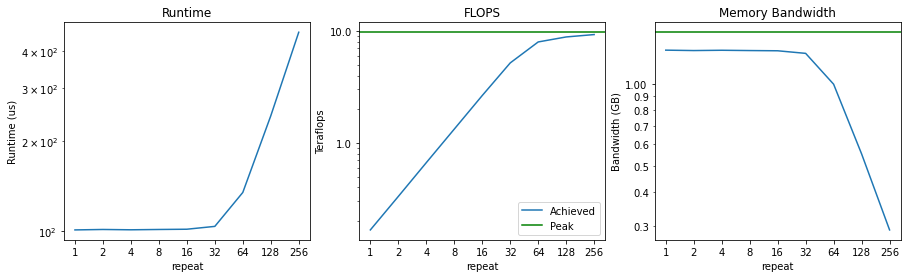
First, notice that the runtime doesn’t increase noticeably at all until we’re performing 64 multiplications. That means that up until that point, we’re mostly memory-bandwidth bound - our compute is mostly sitting idle.
首先注意,在我们做到 64 次乘法之前,运行时间完全没有明显增长。这意味着在那之前我们基本是 memory-bandwidth bound——算力大部分时间都闲着。
As a result, we start off by achieving a measly 0.2 teraflops. As we double the compute intensity, this number grows linearly, until we get close to our peak of 9.75 teraflops . Once we’re close to our peak teraflops, we are considered to be “compute bound”.
结果就是,我们一开始只跑出可怜的 0.2 teraflops。随着 compute intensity 翻倍,这个数字线性增长,直到逼近 9.75 teraflops 的峰值。一旦接近峰值 teraflops,我们就认为进入了 “compute bound” 状态。
Finally, you can see that our memory bandwidth achieved starts out near the peak, and as we increase our compute intensity it starts to drop. This is exactly what we should expect, as we’re spending more and more time performing actual compute instead of accessing memory.
最后可以看到,我们达到的 memory bandwidth 一开始接近峰值,随着 compute intensity 提高则开始下降。这正是预期之中的:我们越来越多的时间花在真正的计算上,而不是访问显存。
In this case, it’s easy to see when we’re compute-bound and when we’re memory-bound. For repeat < 32, we’re saturating our memory-bandwidth while our compute is underutilized. Conversely, once repeat > 64, we see that we’re saturating our compute (i.e. achieving close to peak FLOPS), while our utilized memory bandwidth starts to drop.
在这个例子里,很容易看出什么时候是 compute-bound、什么时候是 memory-bound。当 repeat < 32 时,我们是在打满 memory bandwidth,而算力处于闲置状态;反过来,当 repeat > 64 之后,我们开始打满算力(也就是接近峰值 FLOPS),而用到的 memory bandwidth 开始下降。
For larger systems, it’s often more difficult to say whether you’re compute bound or memory-bandwidth bound, often since they contain a mix of compute-bound and memory-bound components.
对于更大的系统,判断自己到底是 compute bound 还是 memory-bandwidth bound 往往更难,因为它们通常混着 compute-bound 和 memory-bound 两类组件。
One common approach to measuring how compute-bound you are is to measure your achieved FLOPS as a percentage of peak FLOPS. For example, if you’re achieving 80% of your peak FLOPS, then you know that you’re at least 80% compute bound, which is pretty good! The rest of your time is probably spent doing memory-bandwidth operations.
衡量自己有多 compute-bound 的一个常见做法,是用实际达到的 FLOPS 占峰值 FLOPS 的百分比。比如,如果你达到了峰值 FLOPS 的 80%,那你至少知道有 80% 是 compute bound 的,这已经相当不错了!剩下的时间大概率花在 memory bandwidth 相关的操作上。
However, in addition to memory-bandwidth costs, there’s one more thing that might cause your GPUs to not go brrrrr.
不过,除了 memory bandwidth 成本之外,还有一样东西可能让你的 GPU brrrrr 不起来。
Overhead
开销
Overhead is when your code is spending time doing anything that’s not transferring tensors or computing things. For example, time spent in the Python interpreter? Overhead. Time spent in the PyTorch framework? Overhead. Time spent launching CUDA kernels (but not executing them)? Also… overhead.
Overhead 指的是你的代码花了时间去做任何既不搬运 tensor 也不做计算的事情。比如,花在 Python 解释器里的时间?overhead。花在 PyTorch 框架里的时间?overhead。花在启动 CUDA kernel 上(但不包括执行它)的时间?同样是……overhead。
The primary reason overhead is such a pernicious problem is that modern GPUs are really fast. An A100 can perform 312 trillion floating point operations per second (312 TeraFLOPS). In comparison, Python is really slooooowwww. Benchmarking locally, Python can perform 32 million additions in one second.
overhead 之所以这么棘手,根本原因是现代 GPU 真的很快。一张 A100 每秒能完成 312 万亿次浮点运算(312 TeraFLOPS)。相比之下,Python 真的很慢很慢很慢。本地 benchmark 下来,Python 一秒只能做 3200 万次加法。
That means that in the time that Python can perform a single FLOP, an A100 could have chewed through 9.75 million FLOPS.
这意味着,Python 做一次 FLOP 的时间里,A100 已经啃完了 975 万次 FLOPS。
Even worse, the Python interpreter isn’t even the only source of overhead - frameworks like PyTorch also have many layers of dispatch before you get to your actual kernel. If you perform the same experiment with PyTorch, we can only get 280 thousand operations per second. Of course, tiny tensors aren’t what PyTorch is built for, but… if you are using tiny tensors (such as in scientific computing), you might find PyTorch incredibly slow compared to C++.
更糟的是,Python 解释器还不是 overhead 的唯一来源——PyTorch 这类框架在你到达真正的 kernel 之前,还有好几层 dispatch。用 PyTorch 做同样的实验,我们每秒只能拿到 28 万次操作。当然,tiny tensor 本来就不是 PyTorch 的强项,但……如果你确实在用 tiny tensor(比如科学计算里),你可能会发现 PyTorch 比起 C++ 慢得离谱。
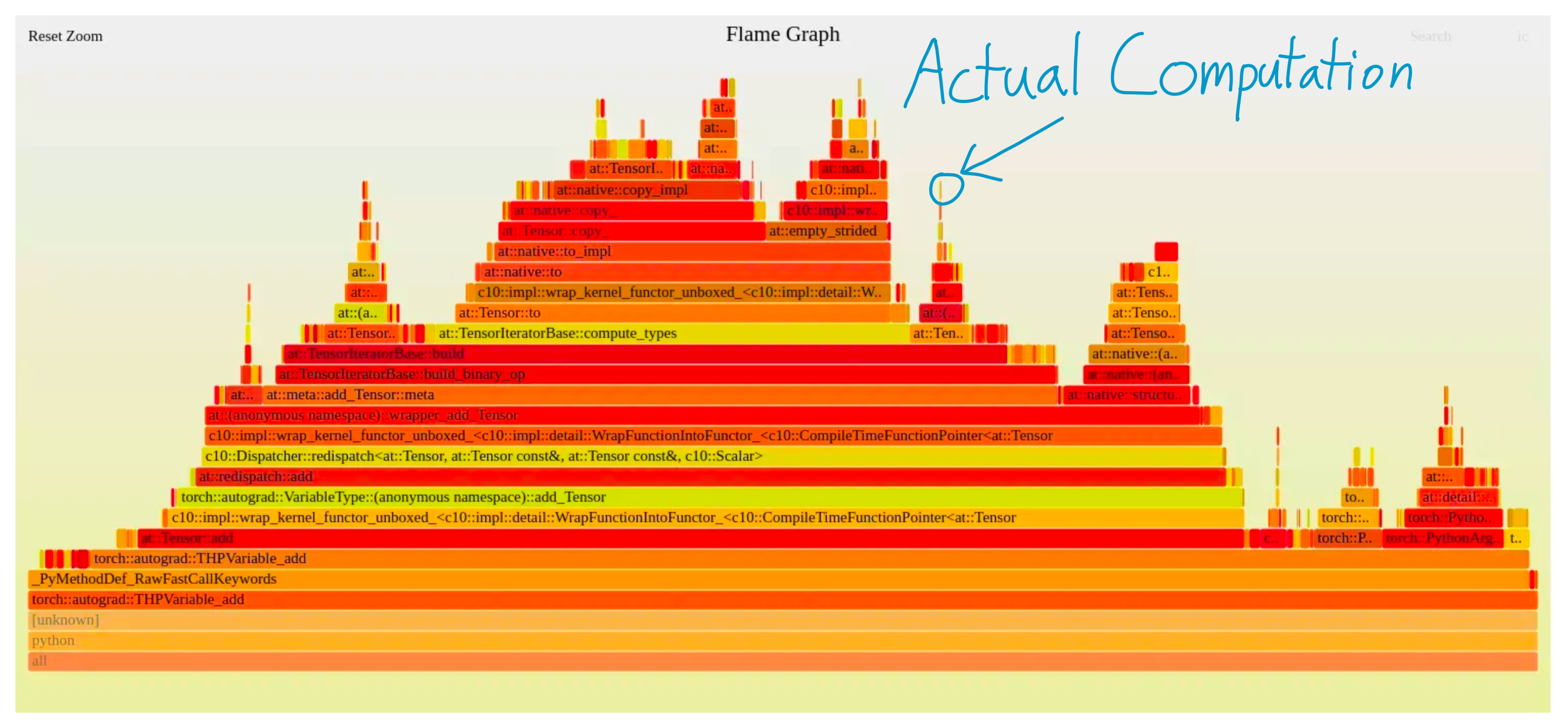
For example, look at this flamegraph profile of PyTorch performing a single addition. That box right there? That’s what’s performing the actual computation. Everything else is pure overhead.
举个例子,看看这张 PyTorch 执行一次加法的 flamegraph 剖面图。就那一小块?那才是真正做计算的部分。其余的全是纯 overhead。
Given this, you might be shocked that anybody uses PyTorch at all, but keep in mind that modern deep learning models are often performing massive operations. Moreover, frameworks like PyTorch execute asynchronously. That is, while PyTorch is running a CUDA kernel, it can continue and queue up more CUDA kernels behind it. So, as long as PyTorch can “run ahead” of the CUDA kernels, most of the framework overhead gets completely hidden!
看到这些,你可能会惊讶居然还有人用 PyTorch。但请记住,现代深度学习模型做的往往是超大规模的运算。而且 PyTorch 这类框架是异步执行的:当 PyTorch 正在跑一个 CUDA kernel 时,它可以继续往后排队更多的 CUDA kernel。所以,只要 PyTorch 能“跑在” CUDA kernel 前面,大部分框架 overhead 就会被完全藏起来!
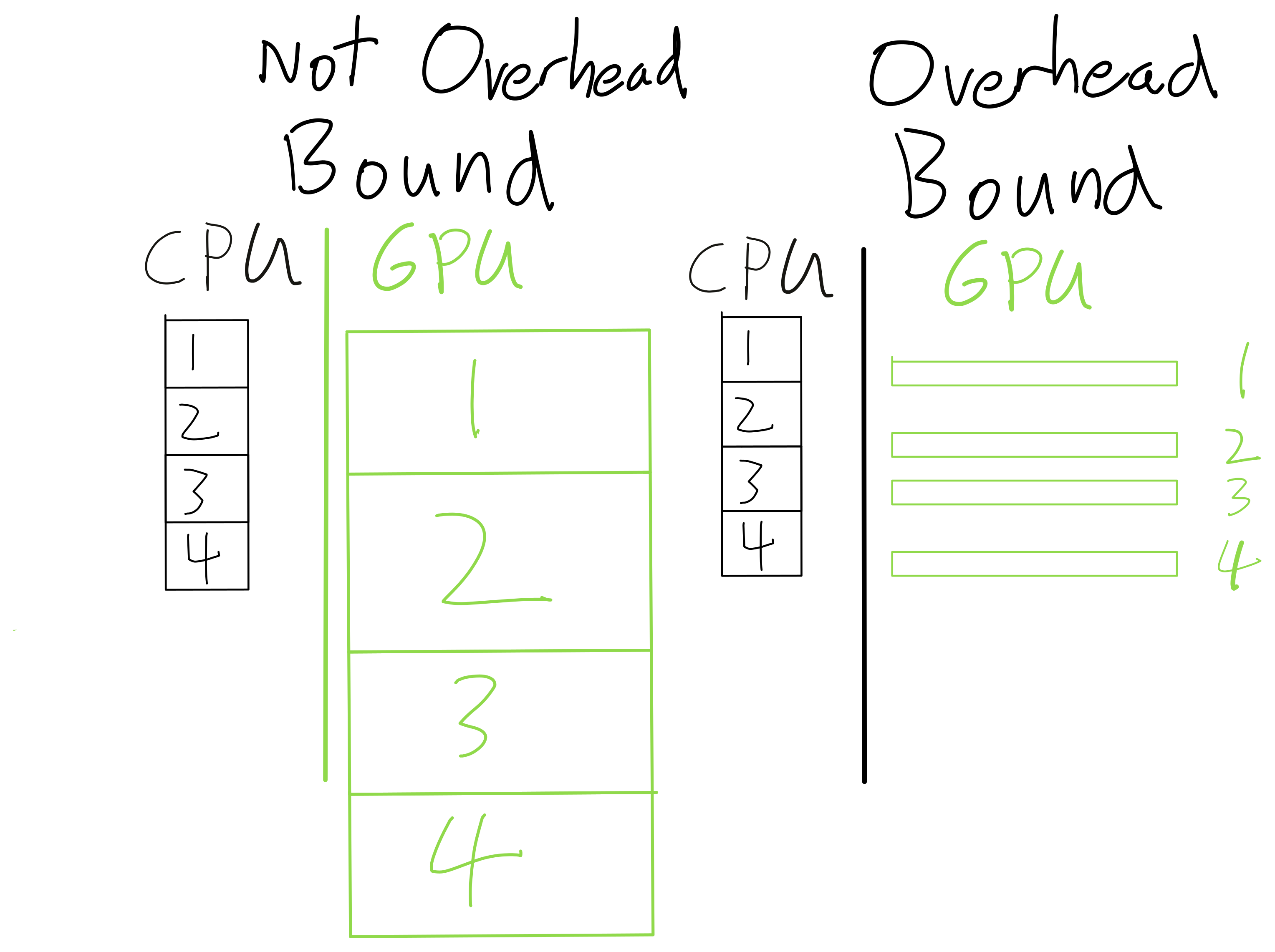
If our GPU operators are big enough, then our CPU can run ahead of the GPU (and thus the CPU overhead is irrelevant). On the other hand, if our GPU operators are too small, then our GPU is going to spend most of its time as an expensive paperweight.
So, how do you tell if you’re in this regime? Well, since overhead generally doesn’t scale with problem size (while compute and memory do), the easiest way to tell is to simply increase the size of your data. If that doesn’t increase the runtime proportionally, you’re overhead bound. For example, if you double your batch size but your runtime only increases by 10%, you’re likely overhead bound.
那怎么判断自己是不是处在这个 regime 里?既然 overhead 一般不会随问题规模增长(而 compute 和 memory 会),最容易的办法就是直接把数据规模调大。如果运行时间没有成比例地增长,那你就是 overhead bound。比如,你把 batch size 翻了一倍,运行时间却只涨了 10%,那多半就是 overhead bound。
Another way is to use the PyTorch profiler. Here, the pink lines actually show how the CPU kernels match up with the GPU kernels.
另一个办法是用 PyTorch profiler。这里粉色的线展示了 CPU 侧的 kernel 和 GPU 侧 kernel 是怎么对应的。
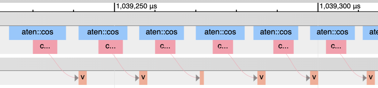
Lots of gaps on the GPU while it's waiting for CPU overhead

Our CPU runs wayyy ahead of the GPU
Another aside - the “GPU-Util” (not “Volatile GPU-Util”) entry in nvidia-smi is basically measuring what percentage of the bottom row is actually running a GPU kernel. So that’s another good way of eyeballing overhead.
再插一句——nvidia-smi 里的 “GPU-Util”(不是 “Volatile GPU-Util”)这一项,基本上就是在测底部那一行里有多少比例真的在跑 GPU kernel。所以它也是目测 overhead 的一个好办法。
The primary reason this overhead exists is due to all of the flexibility frameworks like PyTorch have. Essentially, a lot of time needs to be spent on “figuring out what to do”.
这个 overhead 存在的根本原因,在于 PyTorch 这类框架拥有的各种灵活性。本质上,大量的时间得花在“搞清楚该做什么”上面。
This might be from Python (looking up attributes or dispatching to the right function) or code in PyTorch (all of PyTorch’s dispatcher). For example, when you do a + b, the following steps need to happen.
这可能来自 Python(查属性、分发到正确的函数),也可能来自 PyTorch 的代码(PyTorch 那一整套 dispatcher)。比如,当你写 a + b 时,需要依次发生下面这些步骤。
- Python needs to look up what
__add__dispatches to ona. - PyTorch needs to determine many attributes of the tensor (such as dtype, device, and whether autograd is needed) to determine which kernel to call.
- PyTorch needs to actually launch the kernel.
- Python 需要查出
a上的__add__会分发到哪里。 - PyTorch 需要确定 tensor 的许多属性(比如 dtype、device,以及是否需要 autograd),才能决定调用哪个 kernel。
- PyTorch 需要真正启动这个 kernel。
Fundamentally, this overhead comes from the flexibility of being able to do something different at each step. If you don’t need this flexibility, one way of resolving this flexibility is by tracing it out, like with jit.trace, FX, or jax.jit. Or, alternately, you could do it at an even lower level with something like CUDA Graphs.
从根本上说,这些 overhead 来自“每一步都能做不一样的事”这种灵活性。如果你不需要这种灵活性,那么消化它的一种办法就是把它 trace 出来,比如用 jit.trace、FX 或 jax.jit。或者,也可以在更底层做,比如用 CUDA Graphs。
Unfortunately, this comes at the cost of losing flexibility. One approach I’m excited about that could get us the best of both worlds is to write something more along the lines of a “real” JIT by introspecting at the VM level. See TorchDynamo for more on this.
遗憾的是,这是以牺牲灵活性为代价的。有一个我很期待的方向能让我们两头兼得:在 VM 层面做自省,写出更接近“真正”的 JIT。更多内容可以看 TorchDynamo。
Conclusion
结论
If you want to speed up your deep learning system, the most important thing is to understand what the bottleneck in your model is. That bottleneck determines what the appropriate way of speeding up your system is.
如果你想加速自己的深度学习系统,最重要的一件事就是搞清楚模型的瓶颈在哪。瓶颈决定了什么才是合适的加速手段。
Often, I see researchers and other folks interested in speeding up their PyTorch code try things out blindly without an understanding of what regime you’re in.
我经常看到研究者和其他想加速 PyTorch 代码的人,在不清楚自己身处哪个 regime 的情况下,盲目地各种尝试。
| Performance Regime | Plausible Solutions |
|---|---|
| Overhead-Bound | Tracing, Operator Fusion, don’t use Python, a real JIT :^) |
| Bandwidth-Bound | Operator Fusion |
| Compute-Bound | Use Tensor Cores, give Nvidia more money |
| 性能 Regime | 可能的解法 |
|---|---|
| Overhead-Bound | Tracing、Operator Fusion、别用 Python、上一个真正的 JIT :^) |
| Bandwidth-Bound | Operator Fusion |
| Compute-Bound | 用 Tensor Cores,给 Nvidia 多打钱 |
Of course, arguably, users needing to think about this stuff at all reflects a failure on the part of the framework. PyTorch’s compiler or profile APIs haven’t always been the … easiest to work with, although it is an active area of focus.
当然,也可以说,用户需要操心这些东西本身,就反映了框架的失职。PyTorch 的 compiler 和 profiler API 并不总是……那么好用,尽管这一直是重点投入的方向。
Regardless, I find understanding of basic principles of systems to nearly always be useful - hopefully this was useful to you as well.
无论如何,我认为理解系统的基本原理几乎总是有用的——希望这篇对你也同样有用。
PS: If you like this article, I will be putting much of my future writing at thonking.ai
PS:如果你喜欢这篇文章,我今后的大部分写作都会放在 thonking.ai。
Acknowledgements
致谢
Thanks to Emily Shen, Qian Huang, and folks on EleutherAI for reading earlier drafts of this blog post and providing feedback.
感谢 Emily Shen、Qian Huang,以及 EleutherAI 的朋友们阅读本文的早期草稿并提供反馈。
BibTeX Citation
BibTeX 引用
@article{he2022brrrrfromfirstprinciples,
  author={Horace He},
  title={Making Deep Learning Go Brrrr From First Principles},
  year={2022},
  url={https://horace.io/brrr_intro.html},
}- This might not be what you see on the spec sheet, where it says 19.5 teraflops. The reason for this is that GPUs have even more specialized hardware for fused multiply and add (FMA) instructions. So, for fully general purpose computation, an A100 actually only achieves 9.75 teraflops.
- There are a lot of way to count FLOPS, but this is actually fairly trivial to do in a nice way in PyTorch now - see https://dev-discuss.pytorch.org/t/the-ideal-pytorch-flop-counter-with-torch-dispatch/505
- This isn’t strictly the only reason why increasing batch size might not increase computational time accordingly - in certain regimes it also increases computational intensity. For example, in a MLP you’re typically doing [B, D] x [D, D] matmuls. If B is less than D (say, your batch size is 1 while your hidden dim is 128), then you might negligibly increase your total memory bandwidth, while doubling your compute. I couldn’t figure out a way to explain this nuance easily though.
注释
- 你可能在规格表上看到的不是这个数,那里写的是 19.5 teraflops。原因是 GPU 还有更专门的硬件来处理 fused multiply and add(FMA)指令。所以对于完全通用的计算,一张 A100 实际只能达到 9.75 teraflops。
- 统计 FLOPS 的方法有很多,不过现在用 PyTorch 想漂亮地做这件事其实相当容易——参见 https://dev-discuss.pytorch.org/t/the-ideal-pytorch-flop-counter-with-torch-dispatch/505
- 这并不严格是“batch size 增大而计算时间不按比例增长”的唯一原因——在某些 regime 下,batch size 还会提高计算强度。比如在 MLP 里,你通常做的 [B, D] x [D, D] 矩阵乘法:如果 B 小于 D(比如 batch size 为 1、hidden dim 为 128),那么你的总 memory bandwidth 可能几乎没增加,而计算量却翻了一倍。不过这个细微之处我没能想出一个容易讲清楚的说法。
讨论
这里是静态站点,没有内嵌评论区。如果这篇文章对你有用,欢迎通过 RSS 订阅后续更新。