《走进 Transformer:一个 token 的一生》中英对照全译
Aleksa Gordić 的长文《Inside the Transformer: The Life of a Token》全文对照翻译:左栏英文原文、右栏对应中文。用 Rnj 1.5 的真实结构走一遍前向传播,逐个拆开 RMSNorm、GeGLU MLP、多头注意力、YaRN 与 core attention,并把 KV cache、参数量、FLOPs 和集群规模一次算清。
原文:Inside the Transformer: The Life of a Token,作者 Aleksa Gordić。
本站是中英对照排版:左栏英文原文,右栏对应的中文译文。术语(forward pass、RMSNorm、GeGLU、MHA、YaRN、core attention、KV cache、FLOPs 等)保留英文写法;原文 21 张配图全部保留,并标注出处。
这篇长文用 Rnj 1.5 的真实结构,完整走一遍一个 token 在 transformer 里的前向传播:从分词、embedding,到 32 层里的 RMSNorm、GeGLU MLP、多头注意力,再到 YaRN 位置编码、core attention 的掩码,最后把 KV cache、参数量、FLOPs 和集群规模都算一遍。
In this post, I’ll do a deep dive into the internals of a modern dense transformer [1]. I’ll focus exclusively on the forward pass on a single GPU, as if we were about to perform a training step, while ignoring the backward pass and distributed systems details (in practice, large Transformers are sharded across multiple devices during both training and inference).
这篇文章会深入现代 dense transformer 的内部 [1]。我只讲单张 GPU 上的前向传播——就像我们马上要做一次训练 step 那样——反向传播和分布式系统的细节都略过(实际上,大模型在训练和推理时都会被切分到多张卡上)。
As a running example, I’ll use the exact architecture of Rnj 1.5 - a model I worked on with my team at Ashish Vaswani’s AI Lab (Essential AI Labs).
作为贯穿全文的例子,我会用 Rnj 1.5 的确切结构——这是我在 Ashish Vaswani 的 AI Lab(Essential AI Labs)和团队一起做的模型。
💡 The team behind Rnj-1.5:
Rnj 1.5 could not have happened without an amazing group of people (sorted alphabetically):
Code pod: Adarsh Chaluvaraju, Devaansh Gupta, Yash Jain, Somanshu Singla, Saurabh Srivastava (tech lead), Anil Thomas
STEM pod: Aleksa Gordić (tech lead), Michael Pust, Tim Romanski, Ali Shehper, Kurt Smith (tech lead), Ameya Velingker
Infra pod: Mike Callahan, Philip Monk (tech lead), Khoi Nguyen (tech lead), Alok Tripathy, Yash Vanjani
Org: Divya Mansingka, Mohit Parmar, Peter Rushton
Research and Engineering Roadmap: Ashish Vaswani
💡 Rnj-1.5 背后的团队:
Rnj 1.5 的完成离不开一群非常出色的人(按字母序排列):
Code pod: Adarsh Chaluvaraju、Devaansh Gupta、Yash Jain、Somanshu Singla、Saurabh Srivastava(tech lead)、Anil Thomas
STEM pod: Aleksa Gordić(tech lead)、Michael Pust、Tim Romanski、Ali Shehper、Kurt Smith(tech lead)、Ameya Velingker
Infra pod: Mike Callahan、Philip Monk(tech lead)、Khoi Nguyen(tech lead)、Alok Tripathy、Yash Vanjani
Org: Divya Mansingka、Mohit Parmar、Peter Rushton
Research and Engineering Roadmap: Ashish Vaswani
We announced it this week, with weights released on Hugging Face.
我们这周发布了这个模型,权重已经放到 Hugging Face 上。
It’s a long-context follow-up to Rnj 1.0 [2] that extends the context window from 32k to 160k, scoring 79% on RULER on a 128k context window. This release also offers stronger coding abilities on a wider range of harnesses. See our model card for more details.
This post is structured into seven parts:
本文分成七个部分:
- Transformer forward pass: high-level flow of a token
- RMSNorm: the normalization layer
- GeGLU MLP: GELU-gated feedforward block
- MHA: multi-head self-attention
- YaRN: positional embeddings for long context
- Core Attention: global + block local
- Transformer math: FLOPs/token, cluster sizing, and more
- Transformer forward pass:一个 token 的高层流动过程
- RMSNorm:归一化层
- GeGLU MLP:GELU 门控的前馈块
- MHA:多头自注意力
- YaRN:面向长上下文的位置编码
- Core Attention:global + block local
- Transformer math:FLOPs/token、集群规模估算等
In a follow-up post, I’ll dive into conditional computation, focusing on sparse transformers (MoE).
在后续文章里,我会深入 conditional computation,聚焦稀疏 transformer(MoE)。
As a running example, assume we sample 2 “documents” from a dataset, with:
作为贯穿全文的例子,假设我们从数据集里采样了 2 个“文档”,并且:
- batch size = 1
- sequence length = 16
- document packing enabled
- batch size = 1
- sequence length = 16
- 开启了 document packing
We’ll trace how a token flows through the transformer and, along the way, unpack each component.
我们来追踪一个 token 如何流过 transformer,并沿途把每个组件拆开讲。
Let’s start. Spend some time analyzing the following:
先从这里开始。请花点时间分析下面这张图:
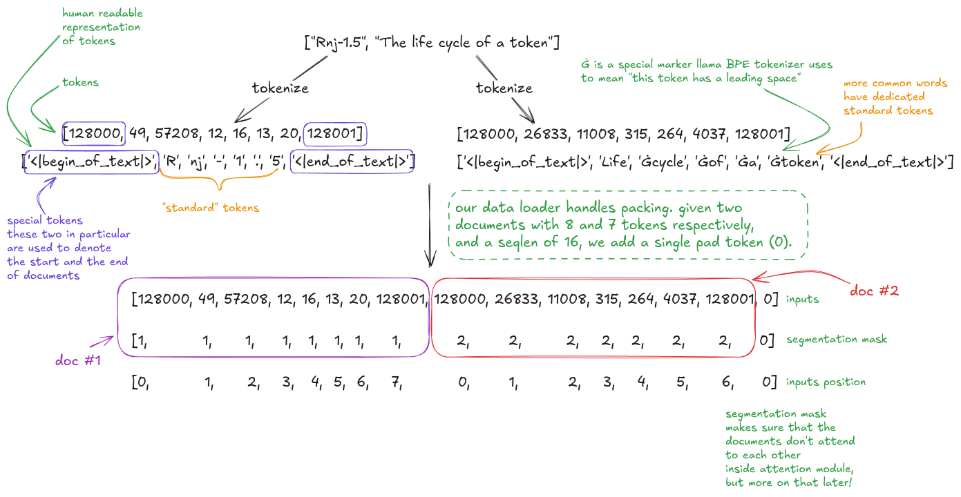
Figure 1: Tokenization stage
We tokenize the documents into sequences of integers, then pack the two documents into a single sequence.
我们把文档分词成整数序列,再把两个文档打包进同一条序列。
For the scope of this blog post, the tokenizer is a black-box component that takes in text and maps it to a sequence of tokens, each represented by an integer ID. In practice, tokenizers are “trained” on a separate corpus of text using algorithms such as BPE, which learn a vocabulary by repeatedly merging frequent character or byte sequences. Good tokenizer design has several desirable properties; for example, representing digits as individual tokens can help with numerical reasoning.
在本文的范围内,tokenizer 是个黑盒:输入文本,输出一串 token,每个 token 用一个整数 ID 表示。实践中,tokenizer 会在一份单独的语料上、用 BPE 之类的算法“训练”出来,通过反复合并高频的字符或字节序列来学出一个词表。好的 tokenizer 设计有几个理想性质;比如把数字拆成单个 token 表示,有助于数值推理。
Alongside the tokens, we construct two supporting structures:
除了 token 本身,我们还要构造两个辅助结构:
- inputs positions - used by the positional embedding module (YaRN)
- segmentation mask - used in attention for masking
- inputs positions —— 供位置编码模块(YaRN)使用
- segmentation mask —— 在 attention 里做掩码
This is the preprocessing stage.
这就是预处理阶段。
📝 Side note:
For efficiency reasons, the data is chunked ahead of time, before training starts, and the data loader feeds these preprocessed structures directly into the training loop. At that point, we never deal with raw strings. The (Spark) data pipelines and the data loader could easily be separate blog posts.
📝 补充说明:
出于效率考虑,数据在训练开始前就已经切好块(chunk),data loader 直接把这些预处理好的结构喂进训练循环。到那时我们再也不碰原始字符串了。(Spark) 数据管线和 data loader 本身都够单独写一篇博客。
Next, we use the input tokens to index into the embedding table.
接下来,我们用输入的 token 去索引 embedding 表。
You can think of the embedding table as the vocabulary of the LLM.
你可以把 embedding 表理解为 LLM 的词表。
This indexing operation converts our sequence of integers into a sequence of 16 4096-dim bf16 vectors:
这次索引操作把整数序列转成 16 个 4096 维的 bf16 向量:
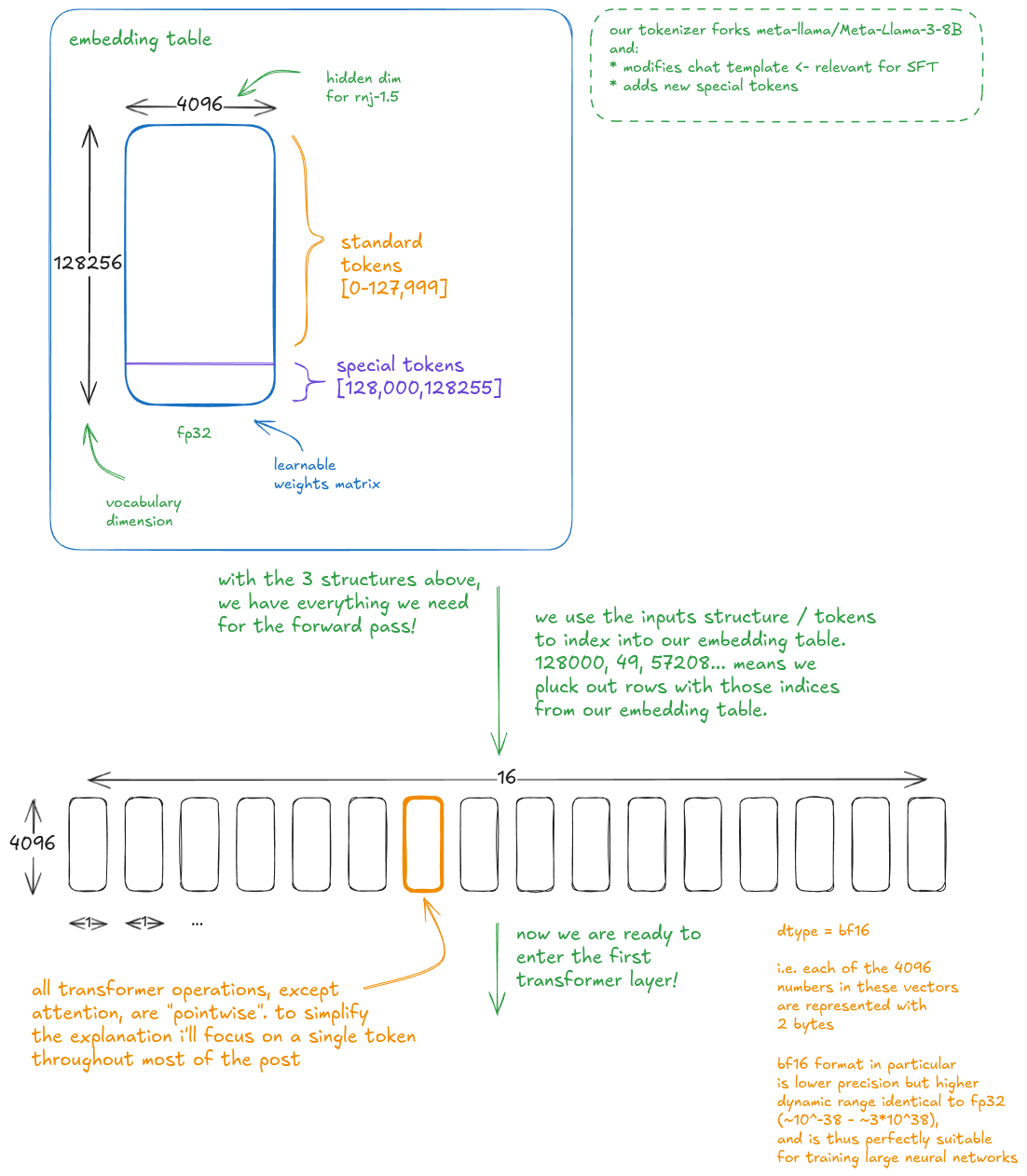
Figure 2: Embedding stage
📝 Side note:
Special tokens don’t naturally appear during tokenization - no text maps to token IDs >= 128,000. They’re injected during training (and later used at inference) to improve performance (e.g. FIM, repo packing, etc.) or to enforce specific behaviors (e.g. end of generation / turn, tool calls).
Let’s dig into FIM [3] (fill-in-the-middle) special tokens.
During (pre)training, we take a document, split it into prefix, middle (infix), and suffix, and construct a sequence of the form:
<FIM_PRE>prefix<FIM_SUF>suffix<FIM_MID>middle. The model is trained to predict the middle given the prefix and suffix. This capability can then be leveraged at inference time.For example, imagine using Rnj 1.5 as an autocomplete model in your favorite IDE. Your cursor naturally splits the code into a prefix and suffix, with the middle missing. By inserting FIM tokens and ending with
<FIM_MID>, you prompt the model to generate a completion for the gap. These tokens help communicate intent to the model.Tokenizer can easily be its own blog post, so I’ll stop here.
📝 补充说明:
special token 不会在分词过程中自然出现——没有任何文本会映射到大于等于 128,000 的 token ID。它们是在训练时被注入的(之后在推理时使用),用来提升性能(比如 FIM、repo packing 等),或者强制某些行为(比如结束生成/结束轮次、工具调用)。
我们来细看 FIM [3](fill-in-the-middle)special token。
在(预)训练阶段,我们取一篇文档,把它切成 prefix、middle(infix)、suffix 三段,构造成
<FIM_PRE>prefix<FIM_SUF>suffix<FIM_MID>middle 这样的序列。模型被训练成:给定 prefix 和 suffix,预测 middle。这项能力之后可以在推理时用起来。举个例子:假设你在喜欢的 IDE 里把 Rnj 1.5 当补全模型用。你的光标天然把代码切成了 prefix 和 suffix,缺的正是 middle。插入 FIM token、并以
<FIM_MID>结尾,就等于提示模型为这段空缺生成补全。这些 token 帮助把意图传达给模型。tokenizer 本身足够单独写一篇博客,这里就打住。
Now we’re ready to enter the first transformer layer.
现在我们准备好进入第一个 transformer 层了。
Note that all transformer layers have (almost) the same structure, so I’ll explain just one. In practice, we pass through 32 such layers - you can think of it as a for loop, but in Rnj 1.5 each layer has its own learnable weights.
注意所有 transformer 层的结构(几乎)都一样,所以我只讲一层。实际上我们要过 32 层——你可以把它想成一个 for 循环,只不过在 Rnj 1.5 里每层都有自己可学习的权重。
“almost” because Rnj-1.5 uses both block-local and global attention layers - the only difference is the mask. At a higher level of abstraction, the statement still holds. More on that in the attention section.
also note that some transformer implementations do weight sharing or partial weight sharing between layers (there are many variations) but here we’re focusing on Rnj 1.5.
“几乎”是因为 Rnj-1.5 同时用了 block-local 和 global 两种 attention 层——唯一的差别只在 mask。抽象层次再高一点,上面的说法依然成立。attention 那节会细讲。
另外注意,有些 transformer 实现会在层与层之间做权重共享或部分权重共享(变体很多),但这里我们只关注 Rnj 1.5。
Let’s do a forward pass through transformer blocks. Analyze the following carefully:
我们来做一次穿过 transformer block 的前向传播。请仔细分析下面这张图:
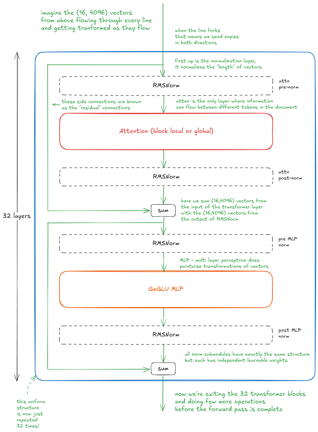
Figure 3: Forward pass through transformer blocks
At a high level, the block consists of four RMSNorm submodules, an MLP, an attention module, two residual connections, and two sum operations. The residual connections simply carry forward copies of vectors from earlier in the block.
从高层看,一个 block 由四个 RMSNorm 子模块、一个 MLP、一个 attention 模块、两条残差连接和两次加法组成。残差连接只是把 block 早期向量的副本原样带过去。
Importantly, all submodules operate on individual vectors, except for attention.
重要的是:除了 attention,所有子模块都作用在单个向量上。
💡 Additional context:
In practice, you’ll find many variations of the transformer block. Design choices include the placement, type and number of normalization layers, the exact MLP structure (gated vs. non-gated, the choice of gating function, etc.), residual connections structure (identity, Attention Residuals [4], etc.), and especially the attention module.
Broadly, attention mechanisms are either quadratic (e.g. MLA [5], scaled dot-product attn, etc.) or linear (e.g. Kimi Linear [6]) in sequence length, each with trade-offs between modeling capacity (especially at long context) and efficiency.
Once the vectors exit the final transformer block, they’re projected into a 128,256-dimensional space via a matrix multiplication. This produces logits, which are converted into a probability distribution via softmax. We sample from it during inference and use it in the cross-entropy loss during training.
向量离开最后一个 transformer block 后,会通过一次矩阵乘法投影到 128,256 维空间。这一步产生 logits,再经 softmax 变成概率分布。推理时我们从中采样,训练时用它算交叉熵损失。
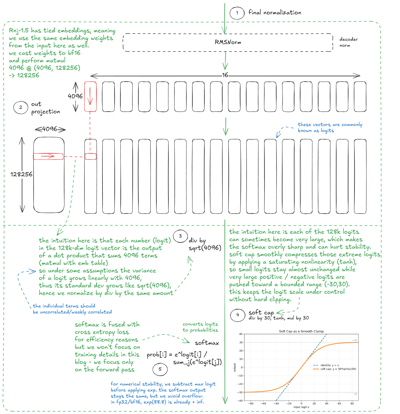
Figure 4:
Next, let’s dive into the individual sublayers. I’ll go in reverse order this time, which conveniently takes us from the simplest to the most complex:
接下来我们逐个深入子层。这次按相反的顺序讲,正好从最简单走到最复杂:
- RMSNorm (Root Mean Square Layer Normalization)
- GeGLU MLP (Multi-Layer Perceptron)
- Attention (Scaled Dot-Product Attention)
- RMSNorm(Root Mean Square Layer Normalization)
- GeGLU MLP(Multi-Layer Perceptron)
- Attention(Scaled Dot-Product Attention)
RMSNorm [7] is a normalization technique used to stabilize the training of deep neural networks.
RMSNorm [7] 是一种归一化技术,用来稳定深度神经网络的训练。
As mentioned earlier, RMSNorm operates on individual vectors, so we’ll focus on a single bf16 4096-dim vector (all others are processed in parallel in the same way). The output has the same shape and dtype:
前面说过,RMSNorm 作用在单个向量上,所以我们只盯一个 bf16 的 4096 维向量(其余向量都并行地做同样处理)。输出的形状和 dtype 都不变:
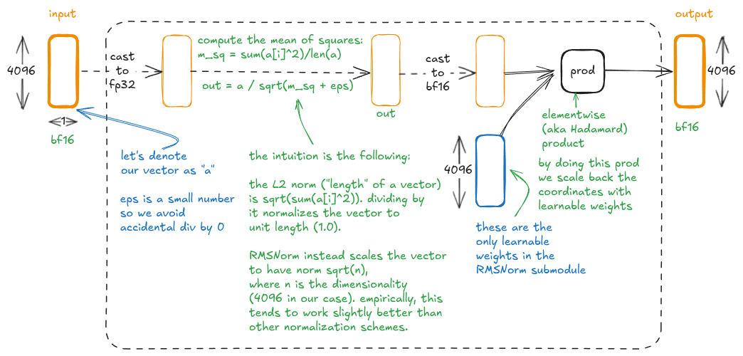
Figure 5: RMSNorm
The MLP is a simple, pointwise feedforward neural network that is used to learn the non-linear relationships between the input and output vectors.
MLP 是一个简单的、逐点(pointwise)的前馈神经网络,用来学习输入向量和输出向量之间的非线性关系。
Our variant is GeGLU (GELU-gated linear unit [8]), where the gating mechanism uses GELU and takes the form W2 @ GELU(W0@X)*(W1@X):
我们用的变体是 GeGLU(GELU-gated linear unit [8]),它的门控机制用 GELU,形式是 W2 @ GELU(W0@X)*(W1@X):
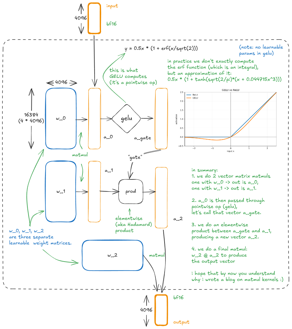
Figure 6: GeGLU MLP
With ReLU, “gate” is more literal because the gating vector is nonnegative, so it only suppresses or scales features. With GELU, gating values can be negative, so the gate can also invert a feature’s sign, which makes “gate” a looser historical term.
用 ReLU 时,“gate”这个词更字面:门控向量非负,所以它只能抑制或缩放特征。而用 GELU 时门控值可以是负的,门还能把特征的符号翻转过来——所以“gate”这个说法更像是个历史遗留的宽松叫法。
MHA is a self-attention mechanism used to model relationships between different tokens in a sequence. We use a special variant of MHA, called GQA, short for group query attention (the number of K/V heads is reduced compared to Q heads, hence multiple queries (group) attend to the same key).
MHA 是一种自注意力机制,用来建模序列中不同 token 之间的关系。我们用的是一个特殊变体 GQA,即 group query attention(K/V head 数量比 Q head 少,因此多个 query 组成一组、关注同一个 key)。
First, I’ll give the high level overview - then we’ll dig into the two most interesting components: YaRN and core attention.
我先讲高层概览,然后深入两个最有意思的组件:YaRN 和 core attention。
We start by mapping each vector independently into query, key, and value vectors. We then reshape them, normalize queries and keys, and apply YaRN (which injects positional information through rotation). Next comes core attention, which mixes information across positions. Finally, we apply a linear projection to produce the output.
我们先把每个向量独立地映射成 query、key、value 向量。然后做 reshape,对 query 和 key 归一化,再施加 YaRN(它通过旋转把位置信息注入进去)。接下来是 core attention,它在不同位置之间混合信息。最后做一次线性投影得到输出。
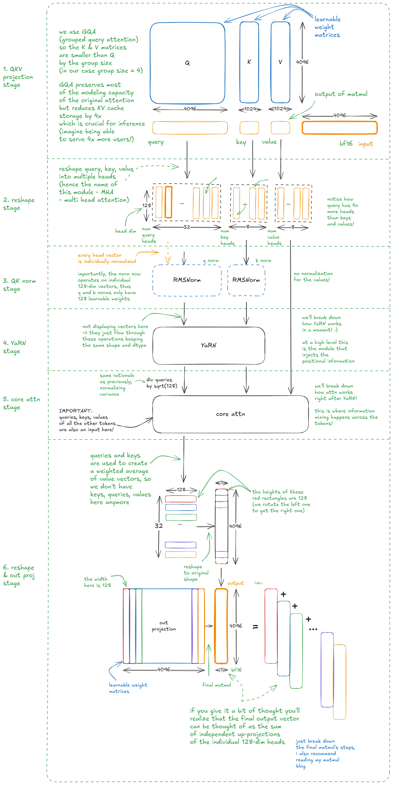
Figure 7: MHA - multi head attention
Let’s now focus on YaRN (Yet another RoPE extensioN).
现在我们聚焦 YaRN(Yet another RoPE extensioN)。
But why do we need positional embeddings in the first place?
但我们为什么需要位置编码?
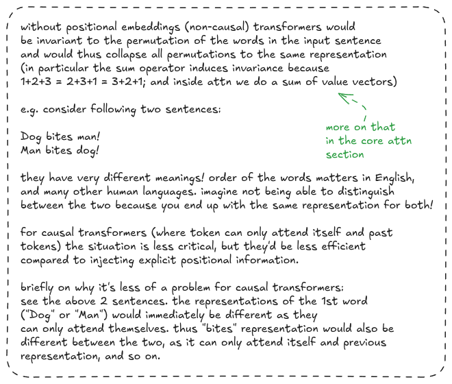
Figure 8: The WHY behind positional embeddings
Now that we understand the why, let’s see how does RoPE work:
理解了为什么,我们再来看 RoPE 是怎么工作的:
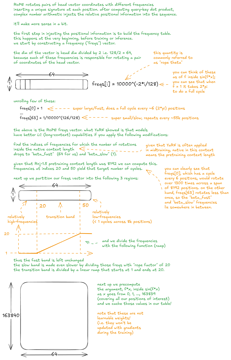
Figure 9: YaRN frequency table
Here is a visualization showing how different YaRN frequencies behave. Notice that our slowest frequency does 1 cycle every 1.088M positions!
这里是一张可视化,展示了不同 YaRN 频率的表现。注意最慢的那个频率每 1.088M 个位置才走完一个周期!
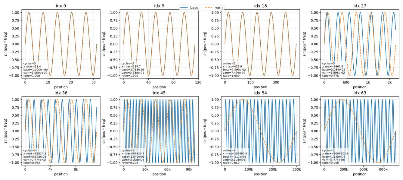
Figure 10: YaRN frequencies
With this we’re ready to see how positional embeddings are injected during the forward pass:
有了这些,我们就可以看前向传播中位置信息是怎么注入的了:
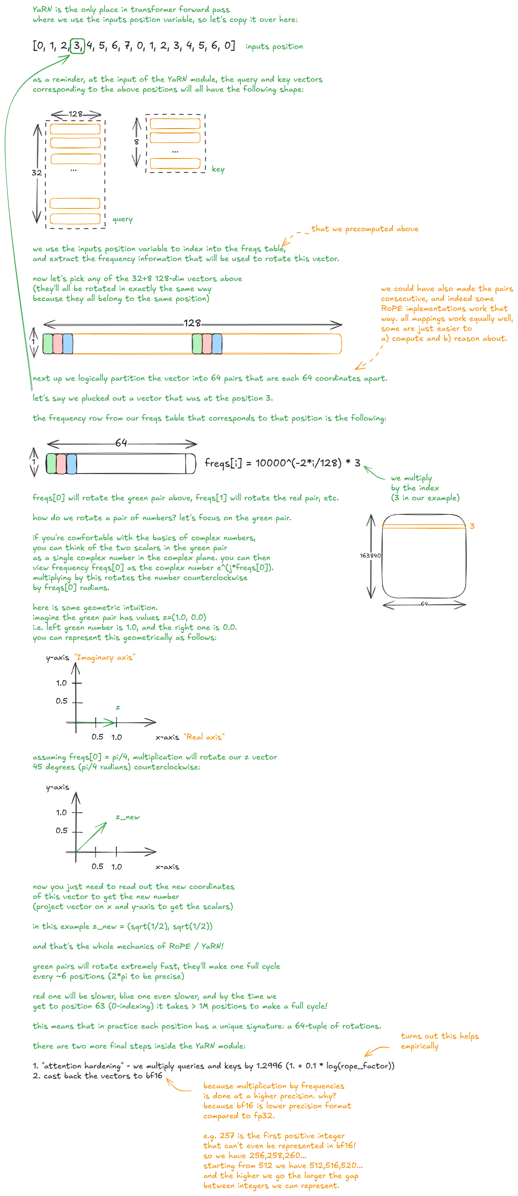
Figure 11: YaRN - forward pass
That wraps up the YaRN forward pass.
YaRN 的前向传播就讲完了。
Now that we understand the mechanics of it you might still be wondering: how does YaRN encode relative positional information via pairwise coordinate rotations of the query and key vectors, followed by a dot product?
理解了它的机制之后,你可能还在想:YaRN 到底是怎么通过对 query 和 key 向量做成对的坐标旋转、再点积,来编码相对位置信息的?
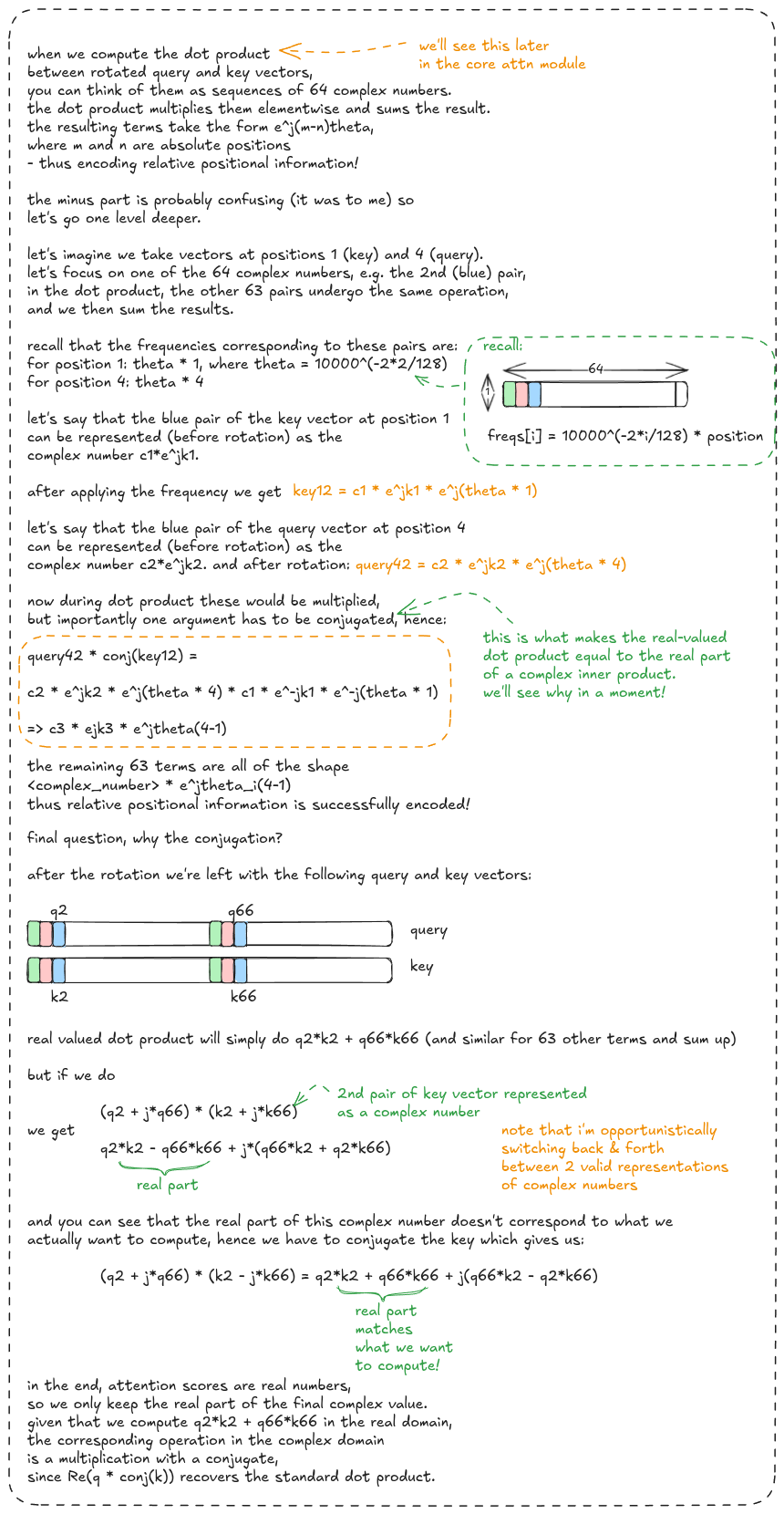
Figure 12: How does RoPE encode relative positional information?
And that’s all there is to RoPE/YaRN! :)
RoPE/YaRN 就全部讲完了!:)
Finally, let’s analyze the core attention mechanism. In practice, we use FlashAttention, which deserves a separate blog post (I actually wrote one back in ’23, check it out[11]). Here, I’ll walk through vanilla attention.
Core attention is the mechanism that models relationships between tokens in a sequence. Take some time to analyze this:
core attention 是建模序列中 token 之间关系的机制。花点时间分析这张图:
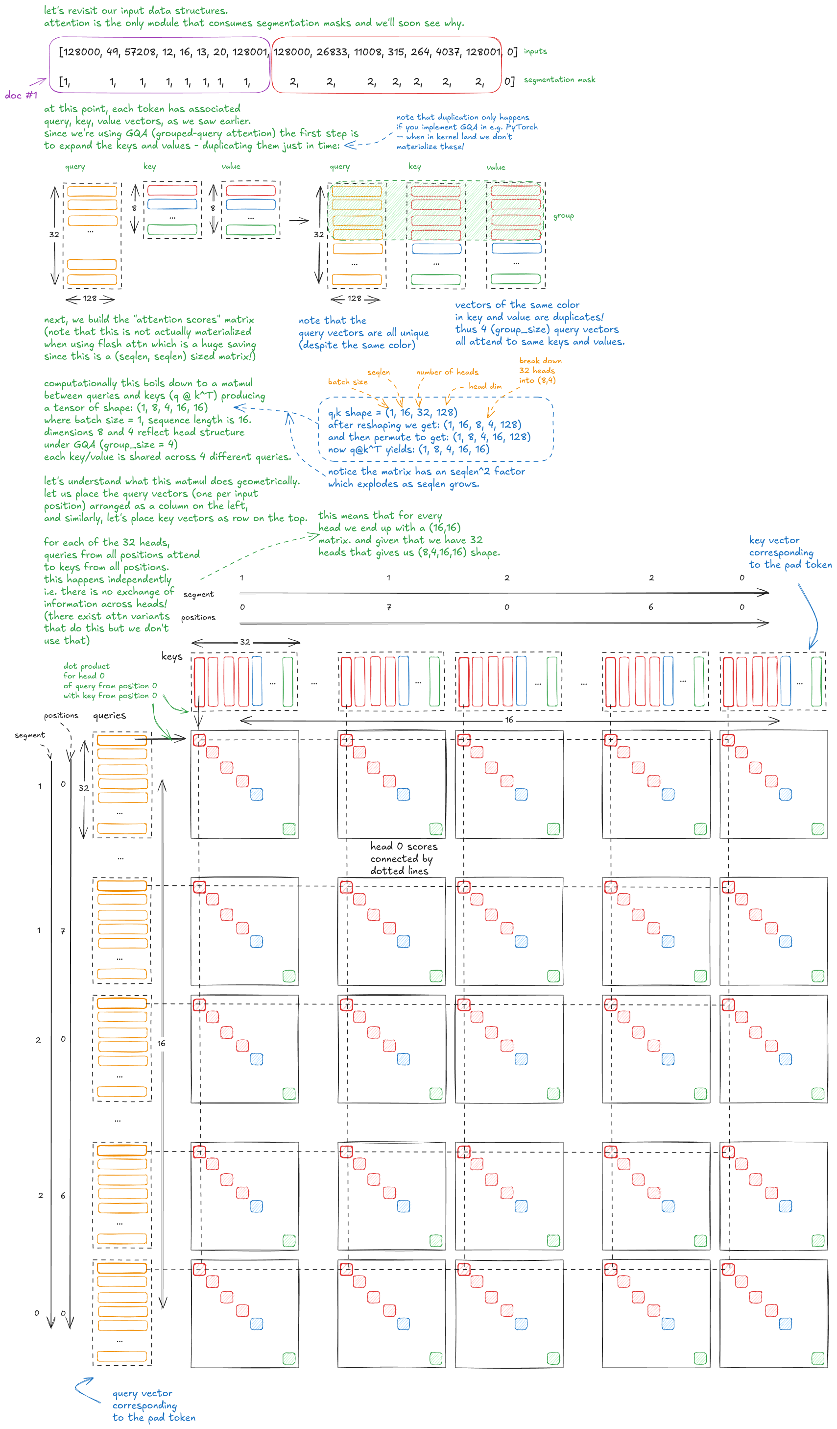
Figure 13: Computing (seqlen, seqlen) matrix of attention scores
Now if we just stopped here we’d have a situation where:
如果就停在这里,我们会遇到两种情况:
- tokens from document 1 could attend to tokens from document 2 (and vice versa)
- token
icould attend to tokeni+1(future token) which breaks the causality
- 文档 1 的 token 能关注到文档 2 的 token(反之亦然)
- token
i能关注到 tokeni+1(未来的 token),破坏了因果性
In order to prevent this we need to introduce masking!
要避免这些,我们必须引入掩码(masking)!
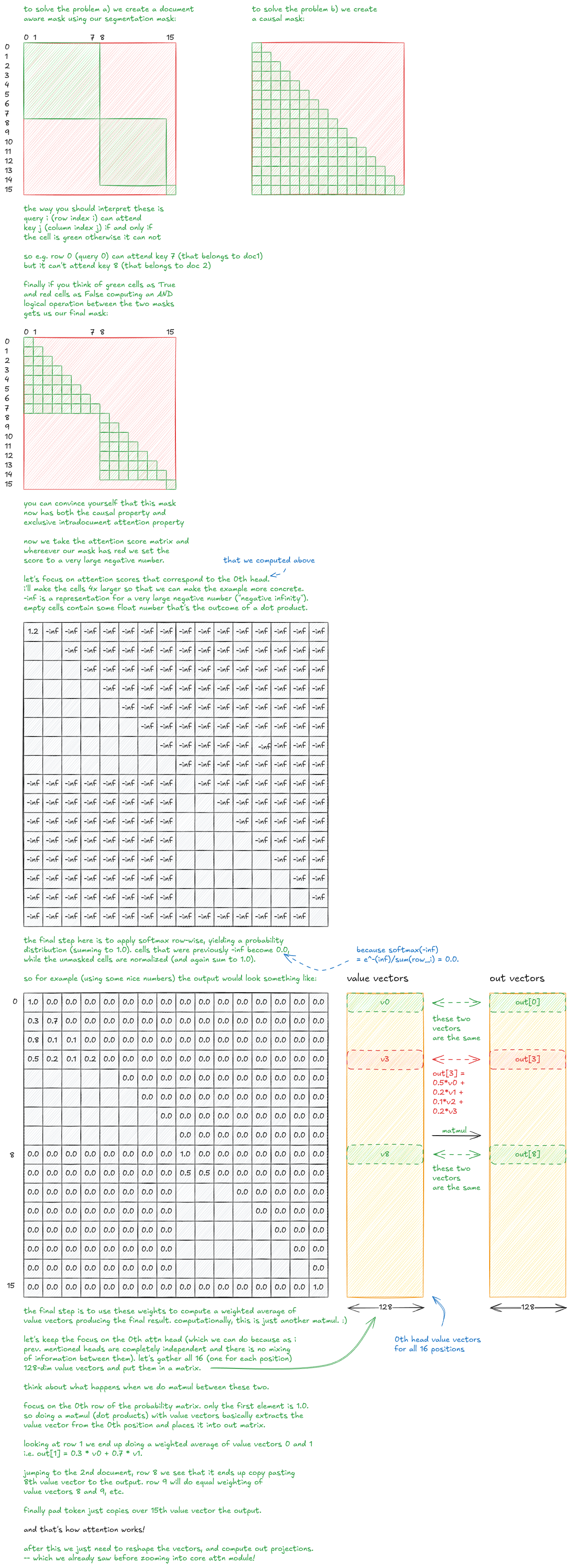
Figure 14: Attention masking & value vector aggregation
Now imagine our sequence length is 32,768 instead of 16. For simplicity, assume a single document with no padding. What would the mask look like?
现在假设序列长度不是 16,而是 32,768。为简单起见,假设只有一篇文档、没有 padding。掩码会长什么样?
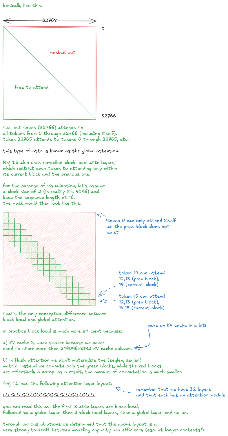
Figure 15: Hybrid attention: block local + global
Here’s another way to visualize the layout, focusing on tokens at positions 9,000 and 10,000:
换一种方式来看这个布局,聚焦位置 9,000 和 10,000 处的两个 token:
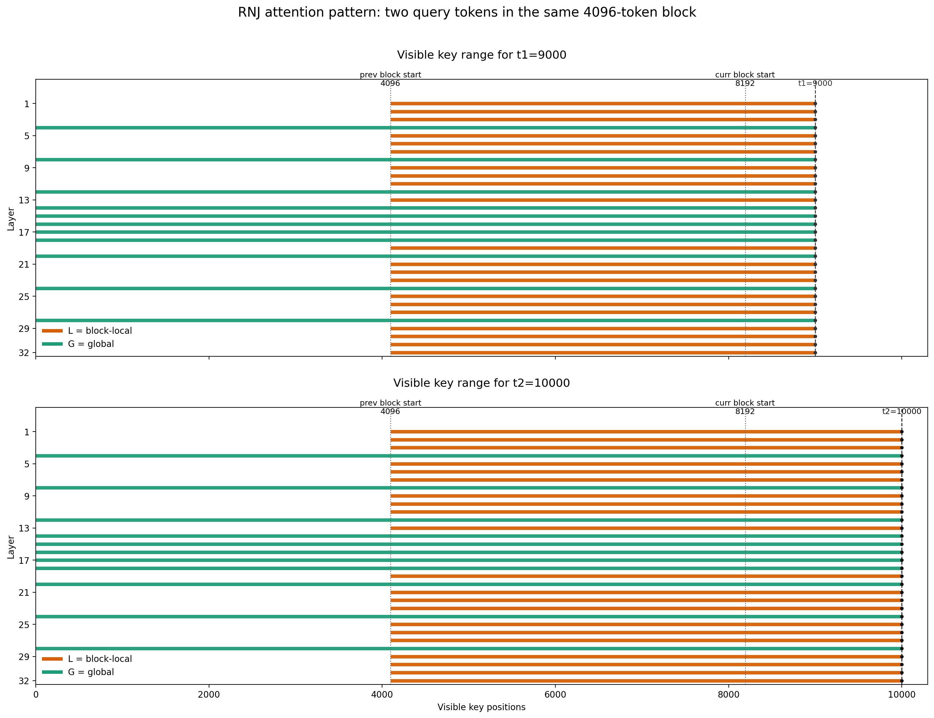
Figure 16: Hybrid attention layout
You can see that in most layers (block-local), these two tokens cannot attend to positions beyond 4,096. In the remaining eight layers (global), they can attend all the way back to position 0.
可以看到,在大多数层里(block-local),这两个 token 能关注的位置不超过 4,096;而在剩下的 8 层里(global),它们可以一路关注回位置 0。
Finally, I want to briefly touch on the KV cache, as it’s an extremely important concept for understanding inference. So far, we’ve looked at the forward pass during training.
最后,我想简单聊聊 KV cache,因为它是理解推理的一个极重要概念。到目前为止,我们看的都是训练时的前向传播。
During inference, transformers are autoregressive - we generate one token at a time. It would be extremely inefficient to recompute the keys and values for all previous tokens at every step. Fortunately, there’s no need: in a causal transformer, they remain unchanged. Instead, we compute them once and store them in a cache.
推理时,transformer 是自回归的——一次生成一个 token。如果每一步都重新计算所有历史 token 的 key 和 value,效率会低到离谱。好在并不需要:在 causal transformer 里,它们不会变。所以我们只算一次,存进 cache。
Let’s go through the basic KV cache storage requirements:
我们来过一遍 KV cache 的基本显存需求:
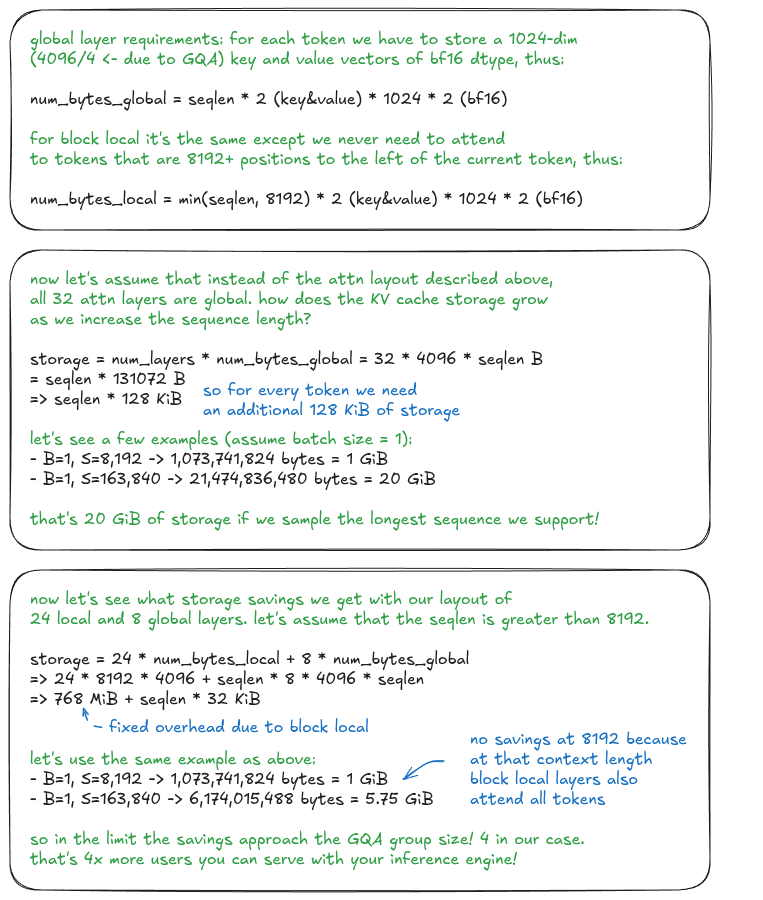
Figure 17: KV cache calculation
Let’s now also calculate how many learnable parameters Rnj 1.5 has. We just need to go through the architecture and account for all the learnable weights.
接着算一下 Rnj 1.5 有多少可学习参数。我们只需要顺着结构把所有可学习权重数一遍。
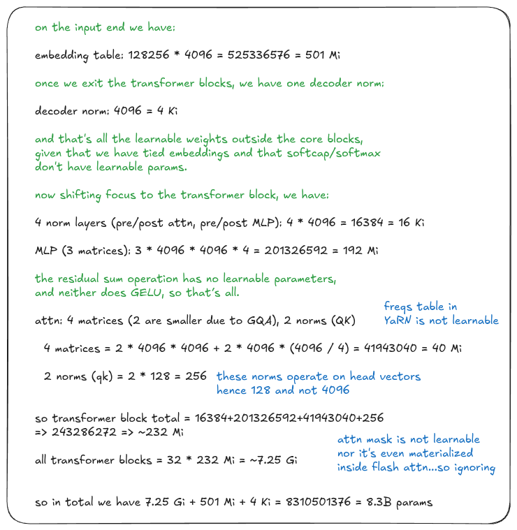
Figure 18: Number of learnable parameters calculation
For quick mental math notice that you only need to account for 3 matrices inside MLP and 4 matrices inside attention and you can ignore everything else.
做口算时注意:你只需要数 MLP 里的 3 个矩阵和 attention 里的 4 个矩阵,其他都可以忽略。
Let’s now calculate how much compute (FLOPs) we need per token. This is extremely valuable when it comes to planning cluster sizing - more on that after this section.
再算一下每个 token 需要多少计算量(FLOPs)。这在规划集群规模时极其有用——这节之后会讲。
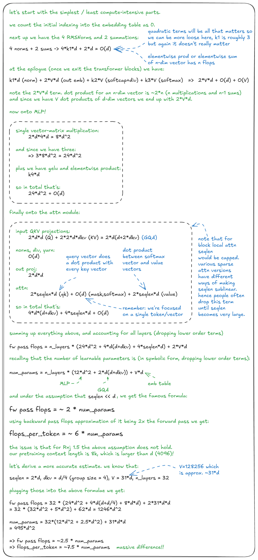
Figure 19: FLOPs/token calculation
It’s worth remembering the 6N formula. It’s also worth remembering the setting under which it holds (i.e. seqlen << inner model dimension).
值得记住 6N 这个公式。也值得记住它成立的前提(即 seqlen << 模型内部维度)。
Finally let’s see how we can use the above formula for cluster sizing:
最后看看怎么用上面的公式估算集群规模:
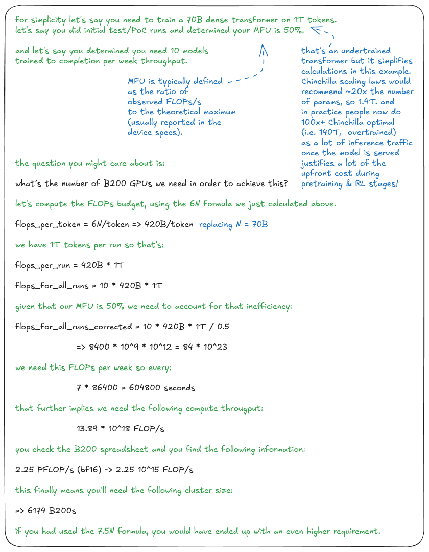
Figure 20: Cluster sizing calculation
You now go to Masayoshi Son and ask for a $1B seed round.
现在你去找孙正义,要一轮 10 亿美元的种子轮。
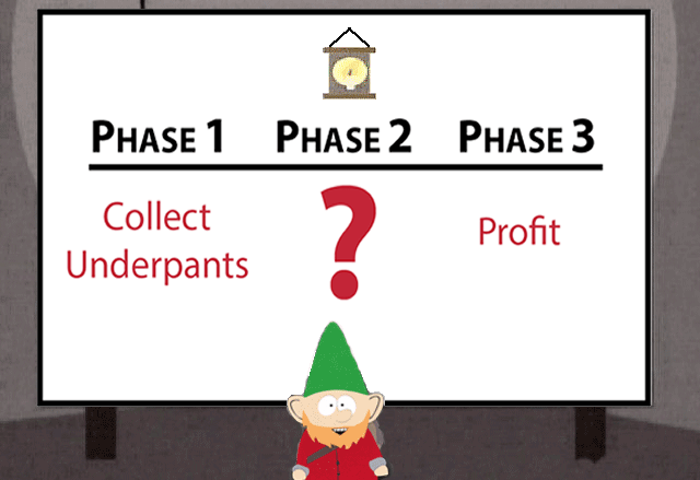
Figure 21: Profit
Epilogue
尾声
We’ve seen how a single token flows through the transformer and how all the subcomponents work together.
我们看到了一个 token 是如何流过 transformer 的,以及各子组件如何协同工作。
We’ve explored YaRN and attention in depth, and derived some of the most important transformer formulas.
我们深入探讨了 YaRN 和 attention,并推导出了一些最重要的 transformer 公式。
💡 Get in touch:
If you spot any errors in the post, please DM me - feel free to drop me a message on X or LinkedIn or via anon feedback.
- “Attention Is All You Need”, https://arxiv.org/abs/1706.03762
- RNJ 1.0, https://essential.ai/research/rnj-1
- “Efficient Training of Language Models to Fill in the Middle”, https://arxiv.org/abs/2207.14255
- “Attention Residual Learning”, https://arxiv.org/abs/2603.15031
- “DeepSeek-V2: A Strong, Economical, and Efficient Mixture-of-Experts Language Model”, https://arxiv.org/abs/2405.04434
- “Kimi Linear: An Expressive, Efficient Attention Architecture”, https://arxiv.org/abs/2510.26692
- “Root Mean Square Layer Normalization”, https://arxiv.org/abs/1910.07467
- “GLU Variants Improve Transformer”, https://arxiv.org/abs/2002.05202
- “YaRN: Efficient Context Window Extension of Large Language Models”, https://arxiv.org/abs/2309.00071
- “RoFormer: Enhanced Transformer with Rotary Position Embedding”, https://arxiv.org/abs/2104.09864
- “Eli5 Flash Attention”, https://gordicaleksa.medium.com/eli5-flash-attention-5c44017022ad
- Muon, https://kellerjordan.github.io/posts/muon/
- “Dissecting Sparsity in Large Language Models: Intrinsic Data-Aware Sparse Attention”, https://arxiv.org/abs/2512.02556
讨论
这里是静态站点,没有内嵌评论区。如果这篇文章对你有用,欢迎通过 RSS 订阅后续更新。